2023 State Elections in Salzburg - A look at data extracted from the electoral lists
Austria
elections
R
How to to scrape content from the electoral lists, and analyze data pertaining to age, regional and gender composition.
1 Preview: Just the results, please!
Note: Best seen in landscape mode on mobile devices. For complete and high resolution images, please see plots in the blogpost.
2 Context
Here’s a purely descriptive blog post on the data contained in the electoral lists for the 2023 State elections in Salzburg, Austria. The code below shows how to download the electoral lists, extract the data of interest, and subsequently look at some hopefully interesting aspects. These include, among others, regional, age, and gender composition of the lists/candidates. I think the graphs speak largely for themselves, so I won’t dig into them at great length.
If you seen any error, have any question etc. don’t hesitate to contact me (best via dm on Twitter or Mastadon).
Fyi - I previously did a similar post for the 2020 elections in Vienna. See here.
3 Get data from electoral lists
Get packages
library(tidyverse)
library(janitor)
library(patchwork)
library(reactable)
library(reactablefmtr)
library(ggh4x)
library(ggtext)
library(patchwork)
library(gghalves)
library(extrafont)
loadfonts(device = "win", quiet = T)
library(hrbrthemes)
library(gt)
library(gtExtras)
The different electoral lists are published on the State of Salzburg’s official website here. First, I’ll get the links for each list.
Code: Extract links to electoral lists
link_main <- "https://www.salzburg.gv.at/pol/wahl/land/ltw23/parteien"

df_links_on_page <- link_main %>%
xml2::read_html() %>%
rvest::html_elements(., "a") %>%
rvest::html_attr("href")  %>%
enframe(name=NULL, value="links")

df_links_list <- df_links_on_page %>%
filter(str_detect(links, "/parteien/")) %>%
distinct() %>%
mutate(links=glue::glue("https://www.salzburg.gv.at{links}"))
Here’s the result:
# A tibble: 7 × 1
  links
  <glue>
1 https://www.salzburg.gv.at/pol/wahl/land/ltw23/parteien/landesliste
2 https://www.salzburg.gv.at/pol/wahl/land/ltw23/parteien/stadt-salzburg
3 https://www.salzburg.gv.at/pol/wahl/land/ltw23/parteien/tennengau-ltw23
4 https://www.salzburg.gv.at/pol/wahl/land/ltw23/parteien/flachgau-ltw23
5 https://www.salzburg.gv.at/pol/wahl/land/ltw23/parteien/pongau-ltw23
6 https://www.salzburg.gv.at/pol/wahl/land/ltw23/parteien/lungau-ltw23
7 https://www.salzburg.gv.at/pol/wahl/land/ltw23/parteien/pinzgau-ltw23
Now, let’s define a scraping function extracting the data from each link/list. Note the \p{C}expression in one of the regex pattern. As it turns out, the websites’ content contains some non-visible characters/signs. The expression matches them. To identify invisible characters in the first place, use stringi::stri_escape_unicode.
Code: Define function extracting data from electoral list
fn_get_tables <- function(link) {

# df_tb1 <- df_links_list$links[[1]] %>%
link %>%
xml2::read_html() %>%
rvest::html_table() %>%
purrr::list_rbind() %>%
rename(
  raw=X2,
  list_position=X1
) %>%
mutate(party=str_extract(list_position, regex("[:alpha:]+")), .before=1) %>%
mutate(party=na_if(party, "")) %>%
mutate(raw=str_trim(raw) %>% str_squish) %>%
mutate(raw=na_if(raw, "")) %>%
fill(., party, .direction="down") %>%
#select(-X1) %>%
mutate(across(.cols=c(party, raw), .fns=\(x) str_remove_all(x, regex("\\p{C}")))) %>%
mutate(across(.cols=c(party, raw), .fns=\(x) na_if(x, ""))) %>%
mutate(nchar_raw=nchar(raw)) %>%
filter(!is.na(raw)) %>%
select(-nchar_raw)

}
Now let’s apply the function.
Code: Apply extract function to each electoral list link
df_table_all <- df_links_list$links %>%
set_names() %>%
map(., fn_get_tables, .progress = T) %>%
purrr::list_rbind(., names_to="list") %>%
mutate(list=str_extract(list, regex("[^\\/]+$"))) %>%
mutate(raw=str_trim(raw)) %>%
filter(!str_detect(raw, regex("^Liste\\s\\d+")))
Below some sample rows of the obtained dataframe. As you can see, the column raw contains all the data from the electoral list, however, in one single string. Candidates’ names, years of birth, places of residence, professions are all lumped together into one cell.
# A tibble: 105 × 4
# Groups:   list [7]
   list           party list_position raw
   <chr>          <chr> <chr>         <chr>
 1 flachgau-ltw23 GRÜNE 18            Dr. med. Fürthauer Bernhard, 1950, Allgem…
 2 flachgau-ltw23 GRÜNE 9             Schöchl MSc Christine, 1972, Diplom Krank…
 3 flachgau-ltw23 GRÜNE 16            Wölflingseder BEd Monika, 1963, Lehrerin,…
 4 flachgau-ltw23 NEOS  3             Feldinger Karin, 1975, Jugendreferentin &…
 5 flachgau-ltw23 GRÜNE 7             Mag.a Stockinger Astrid, 1971, Sozialrefe…
 6 flachgau-ltw23 NEOS  2             Rausch-Mosshammer BA Anna, 1968, Selbstän…
 7 flachgau-ltw23 ÖVP   9             Kaswurm MA BSc Martin, 1986, Geschäftsfüh…
 8 flachgau-ltw23 FPÖ   20            Stöllner Hermann, 1985, Angestellter, 520…
 9 flachgau-ltw23 KPÖ   10            Kelemen Stefan-Denis, 2000, Lehrling, 502…
10 flachgau-ltw23 WIRS  6             Schiestl Josef, 1964, Hüttenwirt, 5161 El…
# ℹ 95 more rows
To disentangle the data, some regular expressions are needed. Below the code.
Code: Split composite string into relevant data
df_table_all_wide <- df_table_all %>%
mutate(
  name=str_extract(raw, regex("^[^,]+")),
  year=str_extract(raw, regex("\\d{4}")),
  origin=str_extract(raw, regex("[^,]+$")),
  profession=str_extract(raw, regex("(?<=\\d{4},).*(?=,\\s\\d{4})"))) %>%
mutate(party=as_factor(party)) %>%
mutate(year=as.numeric(year)) %>%
mutate(list_position=as.numeric(list_position)) %>%
mutate(list=str_to_title(list) %>% str_remove(., regex("-Ltw23"))) %>%
#remove some academic titles to ensure consistency of names across lists
mutate(name_clean=str_remove_all(name, regex("\\S+\\.")) %>% str_trim(., side="both"))
Once the code above is executed, we get a tidy dataframe with the data of interest in separate columns for all candidates. If you want to know e.g. on which lists a specific candidate runs, the table below has you covered.
Code: Tidy Table.
df_table_all_wide %>%
mutate(list_fct=fct(list, levels=lvls_list)) %>%
mutate(age=2023-year) %>%
select(list, party, name, list_position, year, origin) %>%
reactable(,
          columns=list(list=colDef(name="Wahlliste", width=120),
                       party=colDef(name="Partei", width=75),
                       name=colDef(name="KandidatIn", width=250),
                       list_position=colDef(name="Listenplatz",
                                          width=50,
                                          align="center"),
                       year=colDef(name="Geburtsjahr",
                       align="center", width=100),
                       origin=colDef(name="Wohnort", width=150)),
          bordered=F,
          compact = TRUE,
          highlight = TRUE,
          style = list(fontSize = "10px"),
          filterable = TRUE,
          defaultPageSize = 10,
          theme = reactablefmtr::fivethirtyeight()) %>%
          add_title(
            title= html("<p style='font-family:Segoe UI;'>SALZBURG-WAHL 2023: <span style='background-color:black; color:white;list-height:100%;'>Liste aller KandidatInnen</span></p>"),
            font_size=20) %>%
          add_source(source=html("<p style='font-size:8pt; line-height:100%; font-family:Segoe UI;'>Data: https://www.salzburg.gv.at/pol/wahl/land/ltw23/parteien;<br>Analysis: Roland Schmidt | @zoowalk | <span style='font-weight:500'>https://werk.statt.codes</span></p>"))
SALZBURG-WAHL 2023: Liste aller KandidatInnen
Data: https://www.salzburg.gv.at/pol/wahl/land/ltw23/parteien;
Analysis: Roland Schmidt | @zoowalk | https://werk.statt.codes
4 Number of candidates etc
With the data now in the proper format, we can check a few aspects, i.e. the number of candidates per party and list.
Code: Create table
## Function creating barplot

fn_pl_bar_list <- function(list_name) {

# df_table_count <- df_table_all_wide %>%
# count(list_fct, party)

df_table_count <- df_comb %>%
pivot_longer(
  cols=-c(list_fct),
  names_to="party",
  values_to="n"
) %>%
mutate(party=fct(party, lvls_party))

pl_main <- df_table_count %>%
filter(list_fct=={{list_name}})  %>%
ggplot()+
geom_bar(
  aes(
    x=party,
    y=n,
    fill=party),
  stat="identity"
)+
scale_fill_manual(values=vec_party_colors)+
theme_void()+
theme(
  legend.position="none",
  plot.margin=ggplot2::margin(t=20, b=30, unit="pt")
)

if ({{list_name}}=="Landesliste" | {{list_name}}=="Gesamt") {
  pl_main+coord_cartesian(ylim=c(0, max(df_table_count$n)))
} else (pl_main+coord_cartesian(ylim=c(0, 20)))

}

# Create table

df_tbl_df_table_all_wide <- df_table_all_wide %>%
count(list_fct, party) %>%
pivot_wider(
  id_cols=list_fct,
  names_from=party,
  values_from=n
)

df_unique <- df_table_all_wide %>%
distinct(party, name_clean, year) %>%
count(party) %>%
mutate(list_fct="Gesamt") %>%
pivot_wider(
  id_cols=list_fct,
  names_from=party,
  values_from=n
)

df_comb <- df_tbl_df_table_all_wide %>%
bind_rows(., df_unique) %>%
mutate(list_fct=fct_relevel(list_fct, "Gesamt", lvls_list)) %>%
arrange(., match(.$list_fct, levels(.$list_fct))) #sort by levels of factor


pl_df_comb <- df_comb %>%
mutate(graph=list_fct) %>%
gt() %>%
  tab_style(
    style = cell_fill(color = "#e9e9e9"),
    locations = cells_body(rows = list_fct =="Gesamt")
  ) |>
tab_footnote(
  footnote = html("KandidatInnen, nicht Kandiaturen. Personen, die auf mehreren Listen antreten werden nur einmal gezählt."),
  locations=cells_body(columns=list_fct, rows=list_fct=="Gesamt")
) %>%
tab_footnote(
  footnote=html("Abweichende Saklierung der Y-Achse für Bezirkslisten."),
  locations=cells_column_labels(columns=graph)
) %>%
tab_source_note(
  source_note=html(txt_caption_table)
) %>%
tab_header(
  title=html("Salzburg-Wahl 2023:<br><span style='background-color:black; color:white;'>Anzahl KandidatInnen gesamt und pro Liste</span>")
) %>%
cols_align(
  columns = c(list_fct, graph),
  align="left"
) %>%
cols_label(
  list_fct="Liste",
  graph="Graphik",
) %>%
tab_style(
  style=cell_fill(color=vec_party_colors[["SPÖ"]], alpha=0.2),
  locations=cells_body(
    columns=SPÖ,
    rows=SPÖ==7 | SPÖ==5)
) %>%
tab_style(
  style=cell_fill(color=vec_party_colors[["GRÜNE"]], alpha=0.2),
  locations=cells_body(
    columns=GRÜNE,
    rows=GRÜNE==8)
) %>%
text_transform(
  locations=cells_body(columns='graph'),
  fn=function(column) {
    map(column, fn_pl_bar_list) %>%
        ggplot_image(
          height = px(20),
          aspect_ratio = 3)}
) %>%
tab_style(
  style=cell_text(v_align = "middle"),
  locations=cells_body(
    columns=list_fct:MFG
  )
) %>%
tab_options(
table.margin.left = px(0)
) %>%
cols_width(
   ÖVP:MFG ~ px(60)
) %>%
gtExtras::gt_theme_538()

pl_df_comb| Salzburg-Wahl 2023: Anzahl KandidatInnen gesamt und pro Liste |
|||||||||
| Liste | ÖVP | SPÖ | FPÖ | GRÜNE | NEOS | MFG | KPÖ | WIRS | Graphik1 |
|---|---|---|---|---|---|---|---|---|---|
| Gesamt2 | 80 | 67 | 75 | 57 | 28 | 7 | 42 | 26 |  |
| Landesliste | 80 | 62 | 75 | 57 | 27 | 7 | 42 | 26 |  |
| Flachgau | 20 | 20 | 20 | 20 | 14 | 6 | 13 | 10 |  |
| Stadt-Salzburg | 18 | 18 | 18 | 18 | 18 | 7 | 18 | 4 |  |
| Tennengau | 10 | 10 | 10 | 10 | 10 | 6 | 5 | 4 |  |
| Pongau | 10 | 7 | 10 | 10 | 10 | 6 | 6 | 5 |  |
| Pinzgau | 12 | 12 | 12 | 12 | 10 | 6 | 5 | 3 |  |
| Lungau | 10 | 5 | 10 | 8 | 10 | 7 | 5 | 1 |  |
| Data: https://www.salzburg.gv.at/pol/wahl/land/ltw23/parteien Analysis: Roland Schmidt | @zoowalk | https://werk.statt.codes |
|||||||||
| 1 Abweichende Saklierung der Y-Achse für Bezirkslisten. | |||||||||
| 2 KandidatInnen, nicht Kandiaturen. Personen, die auf mehreren Listen antreten werden nur einmal gezählt. | |||||||||
In practical terms, it won’t make any difference, but I found it at least noteworthy that the SPÖ filed a smaller list of candidates on the regional lists for Pongau and Lungau when compared to the ÖVP or the FPÖ. Is this indicative of a recruitment problem?
4.1 List-hopping candiates
Furthermore, the table also suggests that most parties feature candidates which run on more than one regional list. Let’s make this point more clear.
The table below shows for each list and party, and the share of candidates who run exclusively on only one regional electoral list. As it turns out the ÖVP is the only party which maintains a 100 % record across all districts. Also WIRS shows remarkably high numbers. On the other extreme, the MFG has only one single candidate who runs exclusively on one regional list. All other MFG candidates put their names on multiple lists. To a lesser degree, but rather striking, also NEOS features relatively low rates for exclusive candidates (with 50 % in the city of Salzburg being the maximum).
Code: Table exlusive and multi-list candiates
df_unique <- df_table_all_wide %>%
filter(list!="Landesliste") %>%
group_by(party, name, year) %>%
summarise(lists=paste(list, collapse=", "),
lists_n=n())  %>%
ungroup()

df_multi <- df_table_all_wide %>%
filter(list!="Landesliste") %>%
left_join(., df_unique, by=c("party", "name", "year"))

df_multi <- df_multi %>%
mutate(lists_n_1=case_when(
  lists_n==1 ~ "1",
  lists_n>1 ~ ">1",
  .default="missing"
)) %>%
mutate(party=fct_relevel(party, lvls_party) %>% fct_rev) %>%
mutate(list=fct_relevel(list, lvls_list))

df_tb_multi <- df_multi %>%
group_by(list, party, lists_n_1) %>%
summarise(n=n()) %>%
pivot_wider(
  id_cols=c(list, party),
  names_from=lists_n_1,
  values_from=n,
  values_fill=0
) %>%
mutate(party=fct_rev(party)) %>%
rename(
  cand_exclusive=`1`,
  cand_mult=`>1`
) %>%
mutate(
  cand_total=cand_exclusive+cand_mult
) %>%
mutate(
  cand_exclusive_share=cand_exclusive/cand_total
) %>%
group_by(list) %>%
arrange(party, .by_group=T)

df_tb_multi <- df_tb_multi %>%
select(list, party, cand_total, cand_mult, cand_exclusive, cand_exclusive_share) %>%
mutate(cand_exclusive_share_pl=cand_exclusive_share) %>%
gt() %>%
tab_header(
  title=html("Salzburg-Wahl 2023:<br><span style='background-color:black; color:white;'>'Exklusive' KandidatInnen auf Regionallisten</span>"),
  subtitle=gt::md("*Exklusive KandidatInnen:* kandidieren nur auf einer einzigen Regionalliste<br>*Mehrfach KandidatInnen:* kandidieren auf mehr als einer Regionalliste")
  ) %>%
cols_align(
  columns = c(party),
  align="left"
) %>%
tab_source_note(
  source_note=html(txt_caption_table)
) %>%
tab_spanner(
  label=html("<span style='text-algin:left;'>Anzahl Kandidat:Innen</span>"),
  columns=c(cand_total, cand_mult, cand_exclusive),
  id=1
) %>%
tab_spanner(
  label=html("Anteil Exklusiver Kandidat:Innen"),
  columns=c(cand_exclusive_share, cand_exclusive_share_pl),
  id=2
) %>%
cols_label(
  cand_exclusive="'Exklusiv'",
  cand_mult="Mehrfach",
  cand_total="Insgesamt",
  cand_exclusive_share="%",
  cand_exclusive_share_pl="Grafik"
) %>%
fmt_percent(
  columns=cand_exclusive_share,
  decimals=1
) %>%
gtExtras::gt_plt_bar_pct(
  column=cand_exclusive_share_pl,
  fill="orange",
  background = "#e1e1e1",
  scaled=F
) %>%
gtExtras::gt_theme_538() %>%
tab_options(
  # table.font.size="80%",
  table.margin.left = px(0)
)

df_tb_multi| Salzburg-Wahl 2023: 'Exklusive' KandidatInnen auf Regionallisten |
|||||
| Exklusive KandidatInnen: kandidieren nur auf einer einzigen Regionalliste Mehrfach KandidatInnen: kandidieren auf mehr als einer Regionalliste |
|||||
| party | Anzahl Kandidat:Innen | Anteil Exklusiver Kandidat:Innen | |||
|---|---|---|---|---|---|
| Insgesamt | Mehrfach | 'Exklusiv' | % | Grafik | |
| Flachgau | |||||
| ÖVP | 20 | 0 | 20 | 100.0% | |
| SPÖ | 20 | 1 | 19 | 95.0% | |
| FPÖ | 20 | 1 | 19 | 95.0% | |
| GRÜNE | 20 | 4 | 16 | 80.0% | |
| NEOS | 14 | 9 | 5 | 35.7% | |
| MFG | 6 | 6 | 0 | 0.0% | |
| KPÖ | 13 | 2 | 11 | 84.6% | |
| WIRS | 10 | 1 | 9 | 90.0% | |
| Stadt-Salzburg | |||||
| ÖVP | 18 | 0 | 18 | 100.0% | |
| SPÖ | 18 | 1 | 17 | 94.4% | |
| FPÖ | 18 | 1 | 17 | 94.4% | |
| GRÜNE | 18 | 5 | 13 | 72.2% | |
| NEOS | 18 | 9 | 9 | 50.0% | |
| MFG | 7 | 6 | 1 | 14.3% | |
| KPÖ | 18 | 2 | 16 | 88.9% | |
| WIRS | 4 | 0 | 4 | 100.0% | |
| Tennengau | |||||
| ÖVP | 10 | 0 | 10 | 100.0% | |
| SPÖ | 10 | 1 | 9 | 90.0% | |
| FPÖ | 10 | 1 | 9 | 90.0% | |
| GRÜNE | 10 | 4 | 6 | 60.0% | |
| NEOS | 10 | 8 | 2 | 20.0% | |
| MFG | 6 | 6 | 0 | 0.0% | |
| KPÖ | 5 | 2 | 3 | 60.0% | |
| WIRS | 4 | 0 | 4 | 100.0% | |
| Pongau | |||||
| ÖVP | 10 | 0 | 10 | 100.0% | |
| SPÖ | 7 | 1 | 6 | 85.7% | |
| FPÖ | 10 | 1 | 9 | 90.0% | |
| GRÜNE | 10 | 4 | 6 | 60.0% | |
| NEOS | 10 | 9 | 1 | 10.0% | |
| MFG | 6 | 6 | 0 | 0.0% | |
| KPÖ | 6 | 2 | 4 | 66.7% | |
| WIRS | 5 | 1 | 4 | 80.0% | |
| Pinzgau | |||||
| ÖVP | 12 | 0 | 12 | 100.0% | |
| SPÖ | 12 | 1 | 11 | 91.7% | |
| FPÖ | 12 | 1 | 11 | 91.7% | |
| GRÜNE | 12 | 4 | 8 | 66.7% | |
| NEOS | 10 | 9 | 1 | 10.0% | |
| MFG | 6 | 6 | 0 | 0.0% | |
| KPÖ | 5 | 2 | 3 | 60.0% | |
| WIRS | 3 | 0 | 3 | 100.0% | |
| Lungau | |||||
| ÖVP | 10 | 0 | 10 | 100.0% | |
| SPÖ | 5 | 1 | 4 | 80.0% | |
| FPÖ | 10 | 1 | 9 | 90.0% | |
| GRÜNE | 8 | 5 | 3 | 37.5% | |
| NEOS | 10 | 9 | 1 | 10.0% | |
| MFG | 7 | 7 | 0 | 0.0% | |
| KPÖ | 5 | 2 | 3 | 60.0% | |
| WIRS | 1 | 0 | 1 | 100.0% | |
| Data: https://www.salzburg.gv.at/pol/wahl/land/ltw23/parteien Analysis: Roland Schmidt | @zoowalk | https://werk.statt.codes |
|||||
4.2 Concentration of list positions
Related, but conceptually distinct, is the question how concentrated are list positions among the running candidates of the same party. Are there only a few individuals who cover most of the positions put on the regional electoral lists? Or are the numbers of list positions rather evenly spread out among running candidates? From the table above we can already infer that the latter is the case with the ÖVP (since there are no candidates who run on multiple regional lists). But what about the others?
To shed light on this aspect, let’s get the Gini coefficients and Lorenz curves.
4.2.1 Gini coefficient
Code: Calculate Gini coefficient, create table
library(ineq)

df_districts <- df_table_all_wide %>%
filter(list!="Landesliste") %>%
count(party, name)  %>%
nest(.by=party)

fn_gini <- function(df, column) {
{{df}} %>%
pull({{column}}) %>%
Gini(x=.)
}

tb_df_districts <- df_districts %>%
mutate(gini=map_dbl(data, .f=\(x, y) fn_gini(df=x, column=n))) %>%
select(party, gini) %>%
arrange(desc(gini)) %>%
gt() %>%
tab_header(
  title=html("Salzburg-Wahl 2023:<br><span style='background-color:black; color:white;'>Concentration of list positions among candidates</span>"),
  subtitle=gt::md("Only regional lists.")
  ) %>%
cols_label(
  gini="Gini-Coefficient"
) %>%
fmt_number(
  columns=gini,
  decimals=2
) %>%
cols_align(
  align="center",
  columns="gini"
) %>%
tab_source_note(
  source_note=html(txt_caption_table)) %>%
gtExtras::gt_theme_538() %>%
tab_options(
  table.margin.left = px(0)
)

tb_df_districts| Salzburg-Wahl 2023: Concentration of list positions among candidates |
|
| Only regional lists. | |
| party | Gini-Coefficient |
|---|---|
| NEOS | 0.42 |
| GRÜNE | 0.25 |
| KPÖ | 0.18 |
| MFG | 0.14 |
| SPÖ | 0.07 |
| FPÖ | 0.06 |
| WIRS | 0.04 |
| ÖVP | 0.00 |
| Data: https://www.salzburg.gv.at/pol/wahl/land/ltw23/parteien Analysis: Roland Schmidt | @zoowalk | https://werk.statt.codes |
|
As expected, the table below shows that the list positions are equally distributed among running ÖVP candidates. It’s Gini coefficient is 0. On the other end of the scale, NEOS with a Gini of 0.42 stands out. Hence, a comparably small group of NEOS candidates accounts for a considerable number of their positions put on the electoral lists.
To get a more nuanced and visual representation, below the Lorenz curves as concentration indicators.
4.2.2 Lorenz curves
NoteDetails on the graph
There are a few things going on in the code which might be worth highlighting for the sake of clarity.
For a better contrast, each facet not only contains the curve of the party in question, but also the Lorenz curves of the other parties. The latter are kept in grey. To achieve this, I used the expand_grid function which returns all combinations nested under a new dummy variable (facet_dummy).
To add the absolute numbers of list positions and candidates to the axis labels, I created two separate labeling functions, which multiply the percentages with the total absolute number of each category. At least to me, this adds some additional perspective/clarity to the graph.
Finally, the axis breaks are defined in such a way, that they highlight the position where the Lorenz curve has the greatest change in its slope. This is taken as an indicator to identify sub-groups with a particularly large share of list positions.
Code: Calculate data for Lorenz curves
df_add <- tibble(
  row_id=rep(0, length(unique(df_table_all_wide$party))),
  party=unique(df_table_all_wide$party),
  lists_share_cum=rep(0, length(unique(df_table_all_wide$party))),
  cand_share_cum=rep(0, length(unique(df_table_all_wide$party))))

df_lc <- df_table_all_wide %>%
filter(list!="Landesliste") %>%
count(party, name, name="lists_n")  %>%
group_by(party) %>%
arrange(desc(lists_n), .by_group=T) %>%
mutate(lists_share=lists_n/sum(lists_n),
lists_share_cum=cumsum(lists_share)) %>%
mutate(cand_share=1/n(),
cand_share_cum=cumsum(cand_share))

df_pl <- df_lc %>%
group_by(party) %>%
mutate(row_id=row_number()) %>%
bind_rows(., df_add) %>%
arrange(row_id, .by_group=T)  %>%
select(party, lists_share_cum, cand_share_cum)

df_pl <- df_pl %>%
group_by(party) %>%
mutate(diff_cand_share_cum=lead(cand_share_cum)-cand_share_cum)  %>%
mutate(diff_lists_share_cum=lead(lists_share_cum)-lists_share_cum)  %>%
mutate(slope=diff_cand_share_cum/diff_lists_share_cum) %>%
mutate(diff_slope=slope-lag(slope)) %>%
mutate(max_diff_slope=max(diff_slope, na.rm=T)) %>%
ungroup()

df_combined <- expand_grid(facet_dummy=unique(df_pl$party), df_pl)  %>%
mutate(y_break=case_when(
  facet_dummy==party & max_diff_slope==diff_slope ~ cand_share_cum,
  .default=NA
))

df_party_positions_N <- df_table_all_wide %>%
ungroup() %>%
filter(list!="Landesliste") %>%
count(party, name="party_positions_N")

df_party_candidates_N <- df_table_all_wide %>%
filter(list!="Landesliste") %>%
distinct(party, name)  %>%
count(party, name="party_candidates_N")

df_combined <- df_combined %>%
left_join(., df_party_positions_N, by="party") %>%
left_join(., df_party_candidates_N, by="party")
Code: Plot curves
library(patchwork)
library(ggtext)

pl_combined <- df_combined %>%
group_split(facet_dummy) %>%
map(.x=., function(x) {

breaks <- x %>%
filter(party==facet_dummy) %>%
filter(!is.na(y_break))

if (str_detect(unique(x$facet_dummy), regex("ÖVP|SPÖ|FPÖ|WIRS|MFG"))) breaks[] <- NA

mult_cand <- x %>%
  filter(facet_dummy==party) %>%
  pull(party_candidates_N) %>%
  unique()

mult_pos <- x %>%
  filter(facet_dummy==party) %>%
  pull(party_positions_N) %>%
  unique()

# print(mult)

x %>%
ggplot()+
geom_line(
  aes(x=lists_share_cum,
  y=cand_share_cum,
  group=party),
  color="lightgrey",
  alpha=0.4
)+
geom_line(
  data=. %>% filter(facet_dummy==party),
  aes(
    x=lists_share_cum,
    y=cand_share_cum,
    group=party,
    color=party),
  alpha=0.4,
  linewidth=.75
)+
scale_color_manual(values=vec_party_colors)+
scale_x_continuous(
  labels=\(x) glue::glue("{scales::percent(x)} ({x*mult_pos})"),
  breaks=na.omit(c(0, breaks$lists_share_cum, 1)),
  # breaks=c(0, NULL, 1),
  guide = guide_axis(n.dodge = 1),
  position="bottom",
  expand=expansion(mult=c(0,0))
  )+
scale_y_continuous(
  labels=\(x) glue::glue("{scales::percent(x)} ({x*mult_cand})"),
  breaks=c(breaks$y_break,1),
  expand=expansion(mult=c(0,0))
  )+
facet_wrap(vars(facet_dummy))+
hrbrthemes::theme_ipsum_rc()+
theme(
  plot.title.position="panel",
  plot.margin = ggplot2::margin(0,1,0,0, "cm"),
  legend.position="none",
  axis.title.y.left=element_blank(),
  axis.text.y.left=element_text(
    size=rel(.7),
    vjust=1),
  axis.line.y.left=element_line(linewidth=0.5, color="grey90"),
  axis.line.x.bottom = element_line(color="grey90"),
  axis.text.x.bottom=element_text(size=rel(.7)),
  axis.title.x.bottom=element_blank(),
  panel.grid.minor.x=element_blank(),
  panel.grid.minor.y=element_blank(),
  strip.placement = "outside",
  strip.text = element_textbox(
    padding = ggplot2::margin(4, 4, 0, 4),
    fill="white",
    color="black",
    hjust=0,
    vjust=.5,
    lineheight = 7,
    size=9,
    face="plain")
    )

    }

)

#add y-axis title
pl_combined[[1]] <- pl_combined[[1]]+
labs(y="Share of\ntotal number\nof distinct\ncandidates\n(absolute number\nin brackets)",
x="Share of total number of regional list positions\n(absolute number in brackets)")+
theme(
axis.title.y.left = element_text(
  angle=0,
  vjust=1.0,
  face="italic",
  hjust=1,
  size=(rel(.7/9*11.5)),
  color="grey30"),
axis.title.x.bottom = element_text(
  face="italic",
  size=(rel(.7/9*11.5)),
  color="grey30")
)


pl_all <- pl_combined %>% reduce(`+`)

pl_all <- pl_all +
plot_annotation(
  title="Lorenz curves: Concentration of regional list positions among candidates",
  subtitle=str_wrap("Example NEOS: 9 Neos candidates, they are 32 % of all unique Neos candidates on all regional lists, cover in total 53 positions on all regional lists, what amounts to 74 % of all positions filed by Neos. In contrast, each ÖVP candidate covers only one regional list position.", 120),
  caption=txt_caption_graph,
  theme=hrbrthemes::theme_ipsum_rc()+theme(
    plot.title=element_textbox(size=rel(1.2),
    fill="black",
    color="white"),
    plot.margin=ggplot2::margin(0,0,0,0, "cm"),
    plot.subtitle=element_text(
      size=rel(.8),
      color="grey50",
      margin=ggplot2::margin(b=0.2, t=0.05, l=0, r=0, unit="cm")
    ),
  plot.caption=element_markdown(
    color="grey50",
    size=rel(.7)),
  axis.text.y.left=element_text(size=rel(0.3))
  )
)+
plot_layout(ncol=2)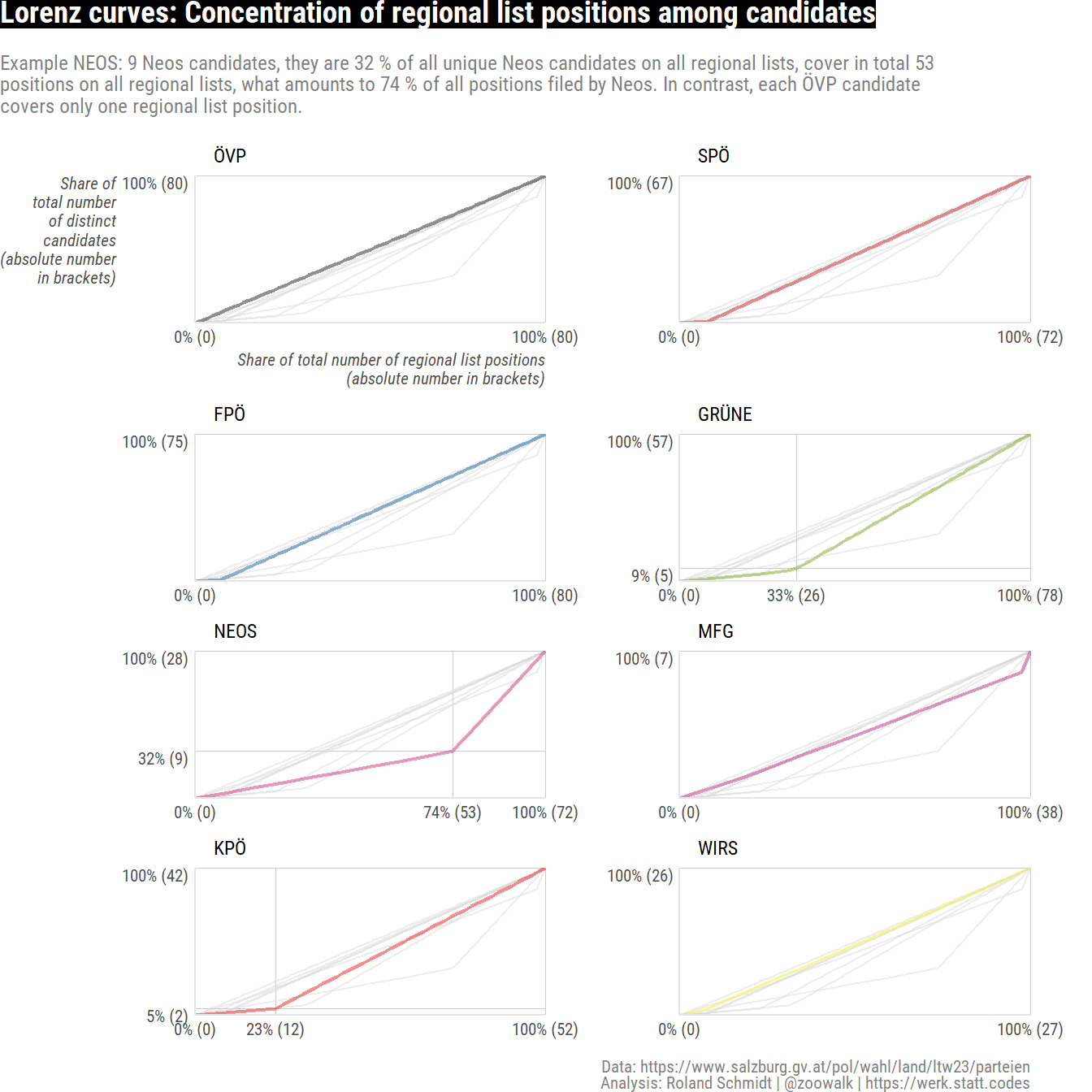
The table and graphs above reveal a considerable concentration of places on the electoral lists among NEOS candidates. As highlighted in the graph, 32 % of all (unique) NEOS candidates across all regional lists cover 74 % of their total regional list positions. For the Greens, 5 candidates (9 %) account for 33 % of all their regional list positions.
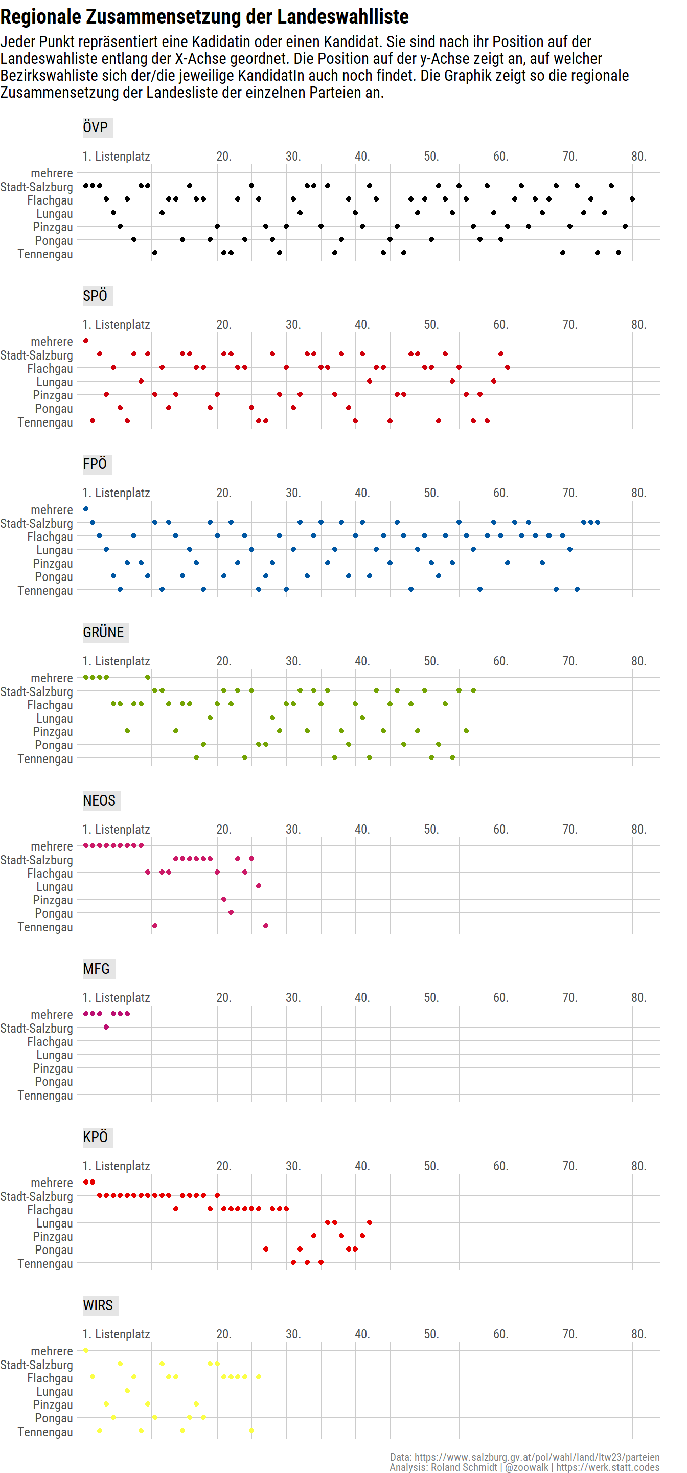
5 Regional Composition of State Electoral list (Landesliste)
In addition to the regional lists, candidates can also run on the state list. One thing which I was curious about was how/whether candidates running on the different regional lists are also featuring on the state’s electoral list. I would assume from an intra-party perspective it could be relevant e.g. when it comes to who shows up where on the state’s list. The graph below visualizes the relation.
A few things which I noticed:
- The sequence of candidates on the state lists of ÖVP, SPÖ, and FPÖ is rather balanced when it comes to the positioning of candidates from the different regional lists. There are only a few instances where candidates running also on the same regional list are positioned next to each other.
- With the exception of the current governor (Landeshauptmann), Wilfried Haslauer (ÖVP), all leading candidates on the state’s electoral list run also on multiple (!) regional electoral lists.
- KPÖ: There is a clear dominance of candidates running also in the city of Salzburg.
Code: Create df detailing regional composition of state electoral list
##take only district lists; if one candidate runs on more than one list "mehere"

df_reg_lists_member <- df_table_all_wide %>%
filter(list!="Landesliste") %>%
group_by(party, name_clean) %>%
summarise(
  lists_all=paste(list, collapse=","),
  lists_n=n()) %>%
mutate(lists_origin=case_when(
  lists_n>1 ~ "mehrere",
  .default=lists_all
))

#join candidates on state list with their data pertaining to district lists
#those candidates on state list who are not also running on a district list are made
#explicit

df_landesliste_lists_member <- df_table_all_wide %>%
filter(list=="Landesliste")  %>%
left_join(., df_reg_lists_member, by=c("name_clean", "party")) %>%
mutate(lists_origin=fct(lists_origin) %>% forcats::fct_na_value_to_level(., level="keine Bezirksliste") %>% fct_relevel(., "mehrere", after=0L) %>% fct_rev)
Code: Create plot
fn_label <- function(x) {
c(paste0(x[1], ". Listenplatz"), paste0(x[-1],"."))
}

txt_subtitle <- "Jeder Punkt repräsentiert eine Kadidatin oder einen Kandidat. Sie sind nach ihr Position auf der Landeswahliste entlang der X-Achse geordnet. Die Position auf der y-Achse zeigt an, auf welcher Bezirkswahliste sich der/die jeweilige KandidatIn auch noch findet. Die Graphik zeigt so die regionale Zusammensetzung der Landesliste der einzelnen Parteien an."

df_landesliste_lists_member %>%
ggplot()+
labs(
  title="Regionale Zusammensetzung der Landeswahlliste",
  subtitle=str_wrap(txt_subtitle, width=110),
  y="Bezirksliste",
  caption=txt_caption_graph)+
geom_point(aes(
  y=lists_origin,
  x=list_position,
  color=party))+
ggh4x::facet_wrap2(facet=vars(party),
ncol=1,
axes="all")+
# coord_flip()+
scale_color_manual(values=vec_party_colors)+
scale_x_continuous(
  position="top",
  limits = c(.5, NA),
  breaks=c(1, seq(20, 80, 10)),
  expand=expansion(mult=c(.01, 0.05)),
  labels=fn_label)+
hrbrthemes::theme_ipsum_rc()+
theme(
  legend.position="none",
  strip.placement = "outside",
  plot.title=element_text(
    size=rel(1.3),
    face="bold",
    margin=ggplot2::margin(b=.2, unit="cm")),
  plot.title.position = "plot",
  plot.subtitle=element_text(
    size=rel(1),
    margin=ggplot2::margin(b=0.3, unit="cm")),
  plot.caption = element_markdown(
    size=rel(.7),
    color="grey50"),
  axis.title.x.top = element_blank(),
  axis.text.x.top=element_text(
    hjust=.05,
    size=rel(.8),
    margin=ggplot2::margin(l=0, unit="pt")),
 axis.title.y.left = element_blank(),
  axis.text.y.left = element_text(
    size=rel(.8),
    vjust=0.5),
  panel.spacing.x = unit(.5, "cm"),
  panel.spacing.y= unit(.5, "cm"),
  plot.margin=ggplot2::margin(t=0.2, b=0, r=0.7, unit="cm"),
  strip.text.x.top=element_textbox(
    size=rel(.9),
    padding = ggplot2::margin(
      t=2,
      r=4,
      b=2,
      l=0,
      unit="pt"),
    fill="grey90",
    color="black",
    hjust=0,
    vjust=.5,
    lineheight = 13,
    face="plain")
)
6 Gender
6.1 Gender ratio
One further aspect I wanted to look into is lists’ gender composition. While not perfect and coming with all sorts of assumptions, I take candidates’ first names to infer their gender by means of the {gender} package. After checking the results, I realized that a few names were off, so I had to correct them manually (Kay, Gabriele, Dominique, Nevin, Nicola).
Code: Get first name
df_table_all_wide <- df_table_all_wide %>%
mutate(name_first=str_extract(name, regex("[^\\s]+$")) %>% str_extract(., regex("^\\p{L}+")))
Code: Get gender
library(gender)
df_name_first <- df_table_all_wide %>%
distinct(name_first) %>%
mutate(gender=gender(name_first, method="genderize"))
Code: Get gender share, create plot.
#fn to capitalize first facet (GESAMT)
fn_labeller_cap <- function(x) {
  c(str_to_upper(x[1]), x[-1])
}

vec_gender_colors <- c("male"="grey", "female"="#f6ae2d")

df_gender <- df_name_first %>%
unnest(gender) %>%
select(name_first, gender) %>%
mutate(gender=case_when(
  name_first=="Kay" ~ "male",
  name_first=="Gabriele" ~ "female",
  name_first=="Dominique" ~ "female",
  name_first=="Nevin" ~ "female",
  name_first=="Nicola" ~ "female",
  .default=gender
))

#join gender with names
df_table_all_wide_gender <- df_table_all_wide %>%
left_join(., df_gender, by="name_first")

df_total <- df_table_all_wide_gender %>%
distinct(party, name_clean, gender) %>%
mutate(list_fct="Gesamt")

df_pl_gender <- df_table_all_wide_gender %>%
bind_rows(., df_total) %>%
mutate(gender=fct_rev(gender)) %>%
mutate(party=fct_rev(party)) %>%
mutate(list_fct=fct(list_fct, levels=c("Gesamt", lvls_list)))

# length(unique(df_pl$list_fct))
strip_backgrounds <- list(element_rect(fill="grey80"))

#create empty list; as many elements as facets
strip_backgrounds <- vector(mode = "list", length = length(unique(df_pl_gender$list_fct)))
strip_backgrounds[[1]] <- element_rect(fill='white', color="white")
strip_text <- vector(mode = "list", length = length(unique(df_pl_gender$list_fct)))
strip_text[[1]] <- element_text(color="black", face="bold")

df_df_gender_label <- df_pl_gender %>%
group_by(list_fct, party, gender) %>%
summarise(n_gender=n()) %>%
mutate(rel_gender_list=n_gender/sum(n_gender)) %>%
filter(gender=="female") %>%
mutate(label_gender=glue::glue("{scales::percent(rel_gender_list, accuracy=0.1)} ({n_gender})"))

df_pl_gender  %>%
mutate(party=fct_relevel(party, lvls_party) %>% fct_rev) %>%
ggplot()+
labs(title=glue::glue("Anteil von <span style='color:{vec_gender_colors[['female']]}'>Frauen</span> je Partei und Wahlliste"),
subtitle=str_wrap("Gender vom Vornamen abgeleitet. In der Kategorie 'Gesamt' werden sämtliche Kandidaturen zusammengefasst, wobei Personen, die auf mehreren Listen kandidieren nur einmal gezählt werden. Absolutzahlen in Klammer.", 110),
caption=txt_caption_graph
)+
geom_bar(aes(y=party,
fill=gender,
group=gender),
color="white",
position="fill")+
geom_text(data=df_df_gender_label %>% filter(rel_gender_list>.2),
  aes(
    y=party,
    x=rel_gender_list,
    label=label_gender
  ),
  size=2.5,
  nudge_x=-0.02,
  hjust=1,
  color="black"
)+
geom_text(data=df_df_gender_label %>% filter(rel_gender_list<=.2),
  aes(
    y=party,
    x=rel_gender_list,
    label=label_gender
  ),
  size=2.5,
  nudge_x=+0.02,
  hjust=0,
  color="black"
)+
geom_vline(
  xintercept=.5,
  linetype="dashed"
)+
scale_x_continuous(
  labels=scales::percent,
  expand=expansion(mult=c(0))
)+
scale_fill_manual(values=vec_gender_colors)+
hrbrthemes::theme_ipsum_rc()+
theme(
  plot.title=element_markdown(
    size=rel(1.2)
  ),
  plot.title.position="plot",
  plot.subtitle=element_text(
    size=rel(.9),
    color="grey50",
    margin=ggplot2::margin(
      b=.3,
      t=.01,
      l=.1,
      r=.1,
      unit="cm")
  ),
  legend.position="none",
  plot.caption=element_markdown(
    size=rel(.7),
    color="grey50"
  ),
  plot.margin=ggplot2::margin(l=0, r=.5, unit="cm"),
  axis.text.x=element_text(size=rel(.8)),
  axis.title.x.bottom=element_blank(),
  axis.title.y.left=element_blank(),
  axis.text.y=element_text(size=rel(.8)),
  panel.spacing.y = unit(.2, "cm"),
  panel.spacing.x = unit(1, "cm"),
  strip.text.x.top=element_markdown(
    margin=ggplot2::margin(
      b=0,
      l=0,
      unit="cm"),
    size=10
  )
  )+
  facet_wrap2(
    vars(list_fct),
    labeller=labeller(list_fct=fn_labeller_cap),
    ncol=3,
    axes="x",
    strip=strip_themed(
      background_x = strip_backgrounds,
      text_x=strip_text)
  )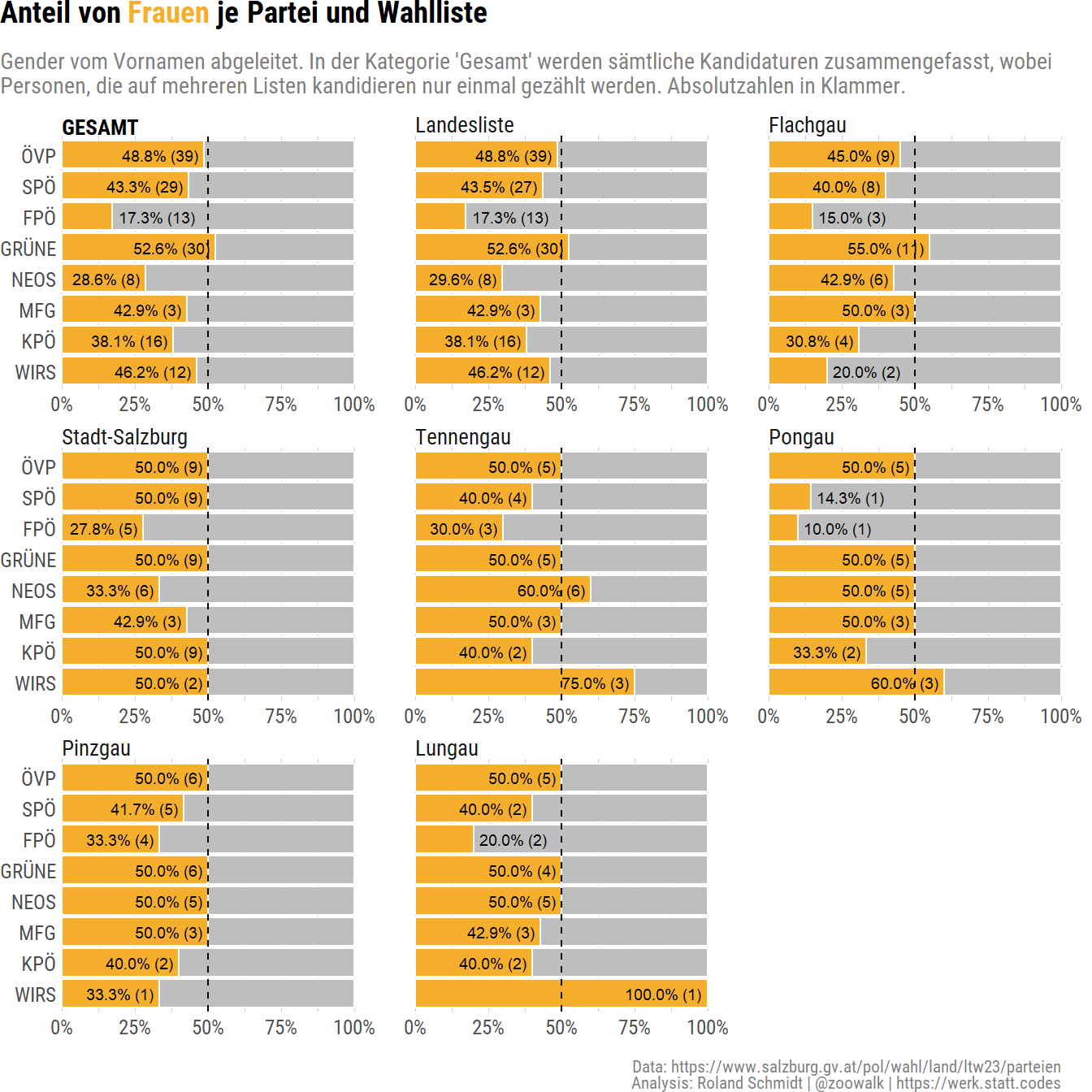
Taking candidates across all lists, ÖVP and Greens have essentially gender parity among their candidates. The FPÖ with only 17.3% female candidates is a stark contrast to its female frontrunner, Marlene Svazek. Somewhat surprising, at least to me, are also NEOS with only 28.6% female candidates.
6.2 Gender & list position
Taking it one step further, the graph below depicts the position of female candidates on the various electoral lists. ÖVP, SPÖ, and Greens have - with minor exceptions - a zipper system when it comes to placing male and female candidates. Out of the eight parties, three feature a female leading candidate on the state list.
Code: List position of female candidates
fn_label <- function(x, sep=NULL, name) {
c(paste0(x[1], {{sep}}, {{name}}), paste0(x[-1],{{sep}}))
}

df_table_all_wide_gender %>%
mutate(party=fct_relevel(party, lvls_party) %>% fct_rev) %>%
mutate(list_fct=fct_relevel(list_fct, lvls_list)) %>%
ggplot()+
labs(
  title=glue::glue("Listenplatz von <span style='color:{vec_gender_colors[['female']]};'>Frauen</span> und <span style='color:{vec_gender_colors[['male']]};'>Männern</span>"),
  subtitle="Gender abgeleitet vom Vornamen.",
  caption=txt_caption_graph,
  x="Listenplatz"
)+
geom_tile(
  aes(y=party,
  fill=gender,
  group=gender,
  x=list_position),
  # shape=22,
  # stroke=2,
  color="white",
  linewidth=1,
  height=0.75
)+
scale_x_continuous(
  position="top",
  limits = c(.5, NA),
  breaks=c(1, seq(10, 80, 10)),
  expand=expansion(mult=c(.0, 0.05)),
  labels=\(x,sep, name) fn_label(x=x, sep=". ", name="Listenplatz")
)+
scale_fill_manual(
  values=vec_gender_colors
)+
hrbrthemes::theme_ipsum_rc()+
theme(
  plot.title=element_markdown(),
  panel.grid.major.y = element_blank(),
  legend.position="none",
  axis.title.y=element_blank(),
  axis.title.x.top = element_blank(),
  axis.text.y.left=element_text(size=rel(.7)),
  axis.text.x.top=element_text(
    hjust=.05,
    size=rel(.7),
    margin=ggplot2::margin(l=0, unit="pt")),
  plot.caption = element_markdown(color="grey30", size=rel(0.7)),
  panel.spacing.y = unit(0.3, "cm"),
  strip.placement = "outside",
  strip.text = element_markdown(
    fill="white",
    color="black",
    size=10,
    lineheight = 2,
    margin=ggplot2::margin(
      l=0,
      b=0,
      r=0,
      t=2,
      unit="pt")),
  plot.margin=ggplot2::margin(l=0, t=0, unit="pt")
)+
facet_wrap2(facet=vars(list_fct),
ncol=1, axes="all")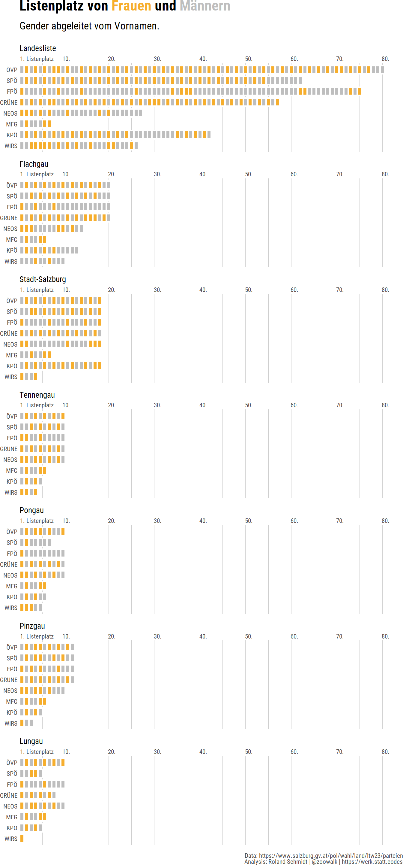
7 Age
The electoral list also contain candidates’ year of birth. Let’s use this as a (not perfect) indicator for age.
7.1 Median age per party across all districts
Code
library(ggbeeswarm)
library(ggiraph)

df_pl <- df_table_all_wide %>%
  group_by(list, party) %>%
  mutate(year_median_list_party=median(year, na.rm=T)) %>%
  mutate(year_mean_list_party=mean(year, na.rm=T)) %>%
  mutate(year_sd_list_party=sd(year, na.rm=T)) %>%
  ungroup()

df_pl_2 <- df_pl %>%
mutate(age=2023-year) %>%
mutate(list_pos=glue::glue("{list_fct} ({list_position})")) %>%
group_by(party, name_clean, year, age) %>%
mutate(list_pos=paste(list_pos, collapse=", ")) %>%
ungroup() %>%
distinct(party, name_clean, year, age, list_pos) %>%
mutate(party=fct_relevel(party, lvls_party)) %>%
mutate(party=fct_rev(party)) %>%
mutate(median_age=median(age, na.rm=T))

pl_age <- df_pl_2 %>%
ggplot(., aes(
  y=party,
  x=age
))+
labs(
title="Salzburg-Wahlen 2023: Alter der KandidatInnen per Partei",
subtitle="Alter über Geburtsjahr approximiert. Partei-Median unterlegt.",
caption=txt_caption_graph
)+
geom_violin(
  color="transparent",
  fill="grey95",
  orientation="y") +
# geom_quasirandom(
#   alpha=0.3,
#   size=.5,
#   groupOnX=FALSE,
#   varwidth = TRUE)+
geom_jitter_interactive(aes(tooltip=glue::glue("{name_clean}
                                                 Geb.Jahr: {year}
                                                 Wahlkreis/Listenplatz: {list_pos}")),
              color="grey50",
              height=0.1,
              alpha=0.4)+
geom_vline(aes(xintercept=median_age))+
annotate(
  geom = "richtext",
  y = Inf,
  x=unique(df_pl_2$median_age)+1,
  label=glue::glue("*Medianalter alle KandidatInnen: {unique(df_pl_2$median_age)}*"),
  color="grey30",
  label.size=unit(0, "lines"),
  label.color=NA,
  hjust=0,
  vjust=1,
  size=3,
  lineheight=1,
  family="Roboto Condensed"
)+
stat_summary(
  geom = "label",
  fun = "median",
  size = 2.5,
  color="white",
  aes(label=after_stat(x), fill=party)
  ) +
stat_summary(
  data= .  %>% filter(party=="WIRS"),
  geom = "label",
  fun = "median",
  label.size=0,
  size = 2.5,
  color="black",
  aes(label=after_stat(x), fill=party)
  ) +
scale_color_manual(values=vec_party_colors)+
scale_fill_manual(values=vec_party_colors)+
scale_x_continuous(
  expand=expansion(mult=c(0.02, 0.01)),
  position="top",
  label=\(x,sep, name) fn_label(x=x, name=" Jahre alt", sep=NULL))+
scale_y_discrete(expand=expansion(mult=c(0, 0.15)))+
hrbrthemes::theme_ipsum_rc()+
theme(
  plot.margin=ggplot2::margin(l=0.5, unit="pt"),
  legend.position="none",
  axis.title.x.top=element_blank(),
  axis.text.x.top=element_text(size=rel(.7)),
  axis.text.y.left=element_text(size=rel(.7)),
  axis.title.y.left=element_blank(),
  panel.grid.major.y=element_blank(),
  plot.title=element_markdown(),
  plot.title.position = "plot",
  plot.subtitle = element_text(
    margin=ggplot2::margin(b=.5, unit="cm")),
  plot.caption = element_textbox(
    color="grey50",
    size=rel(.7)
  ),
  axis.text.y = element_markdown(size=rel(1)),
  axis.text.x = element_markdown(
    size=rel(1),
    hjust=0)
)

giraph_options=list(opts_hover(css =
                               "fill:#FFA500;
                               color:#FFA500"),
                               opts_tooltip(css =
                               "background-color:black;
                               color: white;
                               font-size: 80%;
                               font-family: Roboto Condensed;",
                               offx = 30,
                               offy = -30,
                               delay_mouseout = 1000)
                               )
giraph_height=4
The high median age of Green candidates was quite a surprise to me. Hover over the dots to get details on each candidate.
7.2 youngest & oldest candidates
Finally, to wrap it up, here are the 10 youngest and oldest candidates (since there are ties, the result contains more than 10 individuals.)
Code
df_young <- df_table_all_wide %>%
  ungroup() %>%
  distinct(name, year, party) %>%
  slice_max(., order_by=year, n=10, with_ties=T) %>%
  arrange(desc(year), name) %>%
  mutate(index=dplyr::min_rank(desc(year))) %>%
  mutate(index_name=paste0(index, ". ", name), .before=1) %>%
  select(-index)

df_young  %>%
reactable(.,
columns=list(
  name=colDef(show=F),
  index_name=colDef(
    name="KandidatIn",
    width=200),
  year=colDef(
    name="Geburtsjahr",
    width=100),
  party=colDef(
    name="Partei",
    width=100)),
  details=function(index) {
candidacy  <-  filter(df_table_all_wide, name==df_young$name[index]) %>%
  select(list, list_position)  %>% reactable(.,
  columns = list(list=colDef(width=200, name="Liste"),
  list_position=colDef(name="Listenplatz", align = "center")),
  outline=F, fullWidth=F, compact=T, theme=reactableTheme(style=list(fontSize=12)))
      htmltools::div(style = list(margin = "0px 45px 0px 60px"), candidacy)
  },
  pagination = FALSE,
  onClick = "expand",
  bordered=F,
  compact = TRUE,
  fullWidth = T,
  highlight = TRUE,
  theme=fivethirtyeight(),
  rowStyle = list(cursor = "pointer")) %>%
  add_title(
    title=html("SALZBURG-WAHL 2023: <span style='background-color:black; color:white'>Jüngesten</span> KandidatInnen"), font_size=17) %>%
  add_subtitle(
    subtitle=html("<br>Drop-down zeigt jeweilige Liste & Position an."),
    font_size=11,
    font_weight="normal"
    ) %>%
  add_source(html(glue::glue("<span style='font-style: Roboto Condensed;'>{txt_caption_table}</span>")), font_size=10)
SALZBURG-WAHL 2023: Jüngesten KandidatInnen
Drop-down zeigt jeweilige Liste & Position an.
Data: https://www.salzburg.gv.at/pol/wahl/land/ltw23/parteien
Analysis: Roland Schmidt | @zoowalk | https://werk.statt.codes
Code
df_oldest <- df_table_all_wide %>%
  ungroup() %>%
  distinct(name, year, party) %>%
  slice_min(., order_by=year, n=10, with_ties=T) %>%
  arrange(year, name) %>%
  mutate(index=dplyr::min_rank(year)) %>%
  mutate(index_name=paste0(index, ". ", name), .before=1) %>%
  filter(index<11) %>% #otherwise shows more than 10
  select(-index)

df_oldest  %>%
reactable(.,
columns=list(
  name=colDef(show=F),
  index_name=colDef(
    name="KandidatIn",
    width=200),
  year=colDef(
    name="Geburtsjahr",
    width=100),
  party=colDef(
    name="Partei",
    width=100)),
  details=function(index) {
candidacy  <-  filter(df_table_all_wide, name==df_oldest$name[index]) %>%
  select(list, list_position)  %>% reactable(.,
  columns = list(list=colDef(width=200, name="Liste"),
  list_position=colDef(name="Listenplatz", align = "center")),
  outline=F, fullWidth=F, compact=T, theme=reactableTheme(style=list(fontSize=12)))
      htmltools::div(style = list(margin = "0px 45px 0px 60px"), candidacy)
  },
  pagination = FALSE,
  onClick = "expand",
  bordered=F,
  compact = TRUE,
  fullWidth = T,
  highlight = TRUE,
  theme=fivethirtyeight(),
  rowStyle = list(cursor = "pointer")) %>%
  add_title(title=html("SALZBURG-WAHL 2023: <span style='background-color:black; color:white'>Ältesten</span> KandidatInnen"), font_size=17) %>%
  add_subtitle(
    subtitle=html("<br>Drop-down zeigt jeweilige Liste & Position an."),
    font_weight="normal",
    font_size=11) %>%
  add_source(html(glue::glue("<span style='font-style: Roboto Condensed;'>{txt_caption_table}</span>")), font_size=10)
SALZBURG-WAHL 2023: Ältesten KandidatInnen
Drop-down zeigt jeweilige Liste & Position an.
Data: https://www.salzburg.gv.at/pol/wahl/land/ltw23/parteien
Analysis: Roland Schmidt | @zoowalk | https://werk.statt.codes
# Fin
So that’s it. As always, if you spot any error, have a question etc, don’t hesitate to contact me (best via dm on Twitter or Mastadon).
Reuse
Citation
BibTeX citation:
@online{schmidt2023,
  author = {Schmidt, Roland},
  title = {2023 {State} {Elections} in {Salzburg} - {A} Look at Data
    Extracted from the Electoral Lists},
  date = {2023-04-21},
  url = {https://werk.statt.codes/posts/2023-03-30-sbg-elections-candidate-age/},
  langid = {en}
}
For attribution, please cite this work as:
Schmidt, Roland. 2023. “2023 State Elections in Salzburg - A Look
at Data Extracted from the Electoral Lists.” April 21. https://werk.statt.codes/posts/2023-03-30-sbg-elections-candidate-age/.