Austrian General Elections 2019: Preference votes
elections
stringr
tidyr::pivot
Austria
A look at the distribution of preference votes casted in the 2019 general elections.
1 Context
On 29 September, Austria held its general elections to the national assembly (Nationalrat). By now a flurry of analyses and comments has been published and the caravan of political commentary has largely moved on, at least when it comes to the analysis of the results itself (the government formation train is finally also getting up to speed). One aspect, I personally have never looked into, and which seems to fall a bit under the radar, is the use of preference votes by Austria’s electorate. This post is essentially my first ‘exploratory’ go at preference votes. No specific question, no specific theoretical framework in mind, just poking. I’ll first present the results, then detail some of the steps implemented in R to obtain, analyze and visualize the relevant data. The entire code for the analysis is available on my github account. As always, if you spot any glaring error etc, don’t hesitate and let me know.
Preference vote (Vorzugsstimme) refer to voters’ option (but not obligation) to indicate their support/preference for specific candidates running for the party of their choice. Since Austrian candidates run on a nation wide federal district list (Bundeswahlkreis), one of nine state district lists (Landeswahlkreis), or/and one of 39 regional district lists (Regionalwahlkreis), voters can cast up to three preference votes (here a sample ballot slip). Eventually, a candidate’s number of preference votes can be consequential when it comes to distributing the seats which a party won to the individual candidates. Without preference votes, seats are distributed in accordance to candidates’ position on the electoral list. The lower a candidate is on a list, the lower the likelihood that she can actually get a seat. However, with a sufficient large number of preference votes, the pre-election order on the electoral list can change and initially lower ranked candidates can move up and eventually gain a seat. For details see here.
2 Results
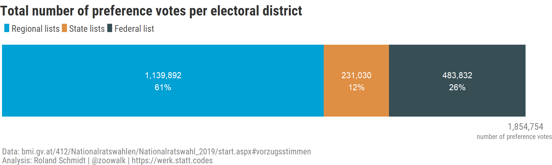
2.1 by district list
Overall, there were 1,8 million preference votes cast. The largest part (more than 60 %) were cast for candidates running on regional district lists. Probably this could be read as voters been particularly keen to support ‘their’ local/regional candidates to make it into the new parliament. Ties between voters and regional candidates are likely to be different than those between voters and candidates running on the more ‘removed’ federal or state constituency list.
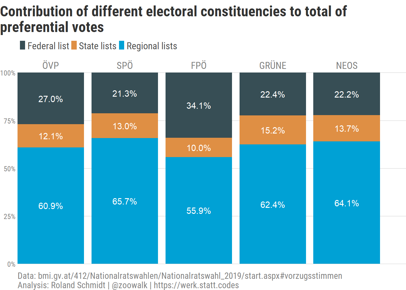
2.2 by constituency list and party
If we further disaggregate these numbers and differentiate between parties, we see that preference votes obtained on the regional level accounted for the majority of preference votes for all parties. However, there is a noticeable difference between the comparable low 55.9 % of the Freedom Party (FPÖ) and e.g. the 65.7 % of the Social Democrats (SPÖ) or the 64.1 % of the NEOS. Or put differently, with 34.1 % the share of preference votes obtained on the federal level, the Freedom Party stands out. As for the underlying reasons, I can only speculate. One reading could be that voters of the FPÖ have weaker ties to their candidates on the regional or state level and hence felt less inclined to cast a preference vote for them. Another one could be that the relation among FPÖ’s candidates on the federal list were particularly competitive and hence a disproportionate high number of voters were mobilized to cast their preference votes on the federal list. Considering the exit of former party leader HC Strache (Ibiza…) and the subsequent (not yet consolidated?) change in the leadership, this seems plausible (see below). It however does not explain why FPÖ voters did not cast preference votes for candidates on state or regional lists.
2.3 Top 5 candidates
If we are interested in candidates, which candidates were particularly successful in securing preference votes?
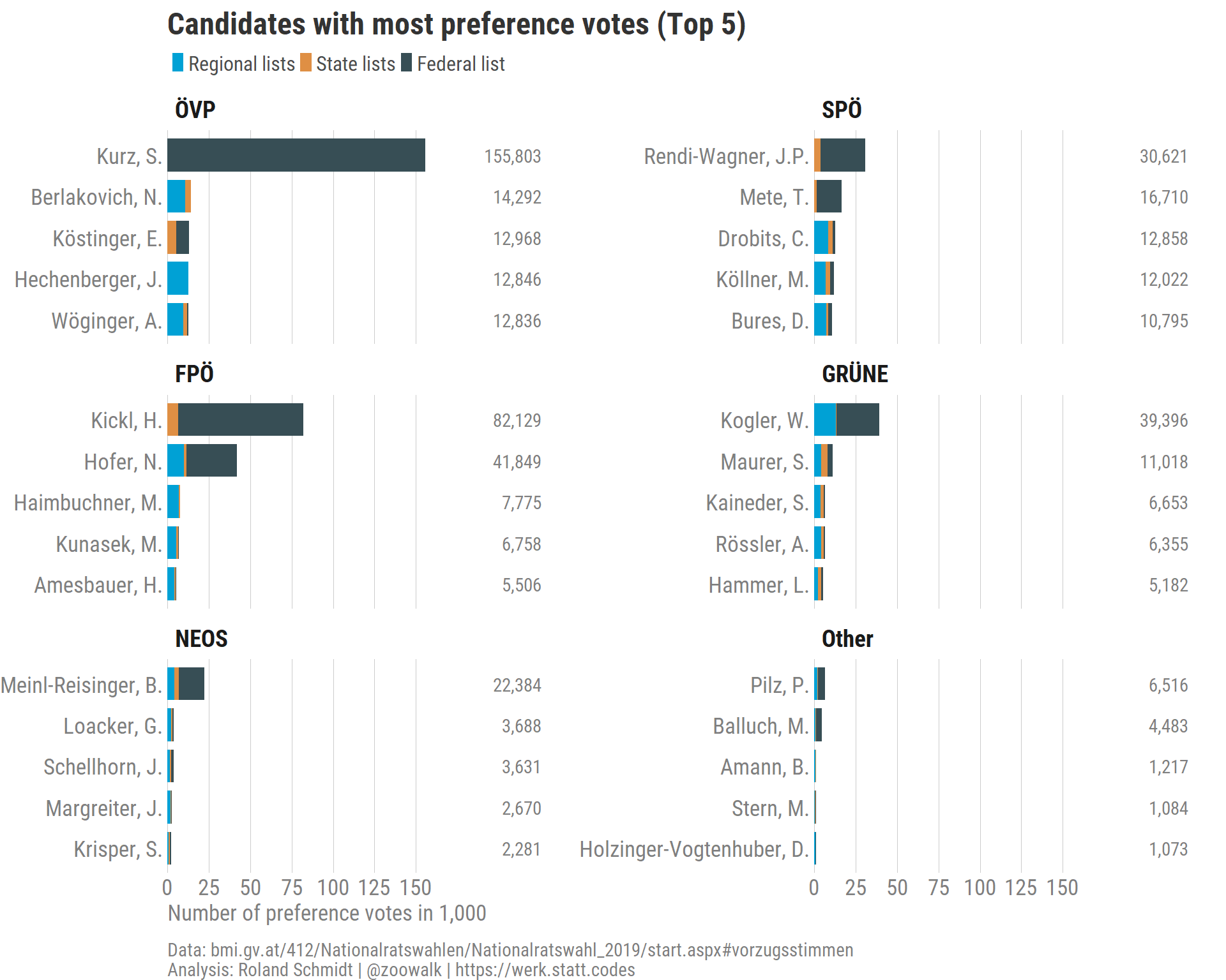
The graph above clearly demonstrates the predominate role of former chancellor Sebastian Kurz when it comes to preference votes. With more than 150,000 votes his result clearly outclasses those of any other candidate. With the notable exception of the FPÖ, the leading candidates/party leaders of all parties succeeded in securing most of the preference votes. In the case of the FPÖ, former Minister of Interior Herbert Kickl overtook his party’s leader, Norbert Hofer. What is also noticeable is that party leaders almost exclusively secured their preference votes from the federal constituency list, while their colleagues largely relied on votes from the regional constituency list.1
Looking at the rankings within parties, I have to admit that I was a bit surprised by the strong performance of a some candidates which I at least had never heard of. The result of T. Mete for the SPÖ, and J Hechenberger for the ÖVP were particularly surprising to me.
2.4 Regional dimension
2.4.1 by district magnitude
The plot below displays a party’s total number of preference votes as percentage of a party’s total vote in each regional electoral constituency. Let’s call this for the sake of easier reference parties’ preference votes - party votes ratio. Or to predend a serious color, P-PVPV ratio.2 This PVPV ratio are grouped by constituencies’ magnitude (number of mandates). The motivation behind is the assumption that the fewer mandates are available the higher will be also intra-party competition. With a smaller cake to distribute (fewer mandates), candidates will try particularly hard to win preference votes and move up the electoral list. Here the analysis is limited to the 39 regional electoral lists. To avoid the indivudal dots overlapping, some random vertical variation was introduced.
The plot seems to provide at least some backing to this proposition. The constituency with only 1 mandate to compete for (Osttirol) features the highest median of parties’ PVPV ratio. While the picture is not entirely clear cut, there seems to be indeed a decreasing median share as constituencies’ magnitude increases from to two to seven mandates. The constituencies with eight and nine mandates (Graz-Umgebung, Hausruckviertel, OberStmk), however, do deviate. Hover over the individual dots to get details.3
2.4.2 by state
If we are interested in whether there are any regional differences when it comes to parties’ PVPV ratios, grouping them by states can be of some help. As the boxplots below show, on average parties’ PVPV ratio was the largest in Burgenland followed by Vorarlberg. These two states are Austria’s two smallest in terms of population. On the other end, Upper Autria (Oberösterreich), Lower Austria (Niedrösterreich), Styria (Steiermark), and Vienna featured on average clearly lower PVPV ratios. These states are Austria’s largest. This difference would be in line with the proposition that candidates in smaller states are better in mobilizing personal support, i.e. preference votes. Closer candidate-voter relations due to smaller population size sounds rather probable to me. But this would certainly need further analysis to corroborate the claim.
2.5 Intra-party dynamics
As already outlined above, preference votes are first and foremost interesting from an intra-party perspective. With sufficient votes, candidates which embarked on the electoral campaign from a lower ranked position can move up the intra-party ladder and secure a seat.
So when do candidate’s move up the ballot list?4
- On the federal level: when a candidate got a preference votes of at least 7 % of those who voted for her party.
- On the state level: when a candidate got preference votes of of at least 10 % of those who voted for her party, or at least as many preference votes as the ‘electoral number’ (Wahlzahl)5.
- On the regional level: when a candidate got preference votes by at least 14 % of those who voted for her party.
Did this happen often?
2.5.1 Candidates’ preference vote party vote ratio
The graph below presents candidates’ preference votes - party votes ratio, or, to stay serious clumsy, C-PVPV. This ratio is candidates’ number of preference votes expressed as % of the total number of votes of her party (in the respective constituency/list). The vertical red lines indicate the stipulated thresholds which candidates have to pass in order to move up on the party’s electoral list. Hover over the individual points to get the data pertaining to each candidate. Note that the x-axis is log-transformed to ensure candidates with low C-PVPV ratios remain (somewhat) visible. Note also that only those candidates are included which actually obtained at least one preference vote.
While the graph provides plenty of details, a few general things standout. First, on the federal level, only two candidates crossed the threshold. Former chancellor Kurz (ÖVP) and former Minister of Interior Kickl (FPÖ). Second, on the state level, not a single candidate secured sufficient preference votes. However, there are several candidates running on regional lists who were able to cross the pertaining threshold. Note that there is no district in which more than one candidate from one party crossed the threshold.
2.5.2 Candidates’ preference votes and electoral number
Aside from candidates’ preference-vote party-vote ratio, candidates have one further avenue to be promoted. See point two of the conditions listed above. On the state constituency level, candidates can move up the ladder not only if they crossed the 10 % threshold, but also if they would have reached more preference votes than the electoral number. The graph below presents the pertaining figures. In short, none of the candidates succeeded in doing so in these elections. In fact, candidates are pretty far from this threshold.
Code
state_electoral_number_plot_interactiveWith the above, we know by now who was able to muster sufficient preference votes to cross the relevant thresholds. However, when aggregating, it makes sense to differentiate between list leaders and those of lower ranks.
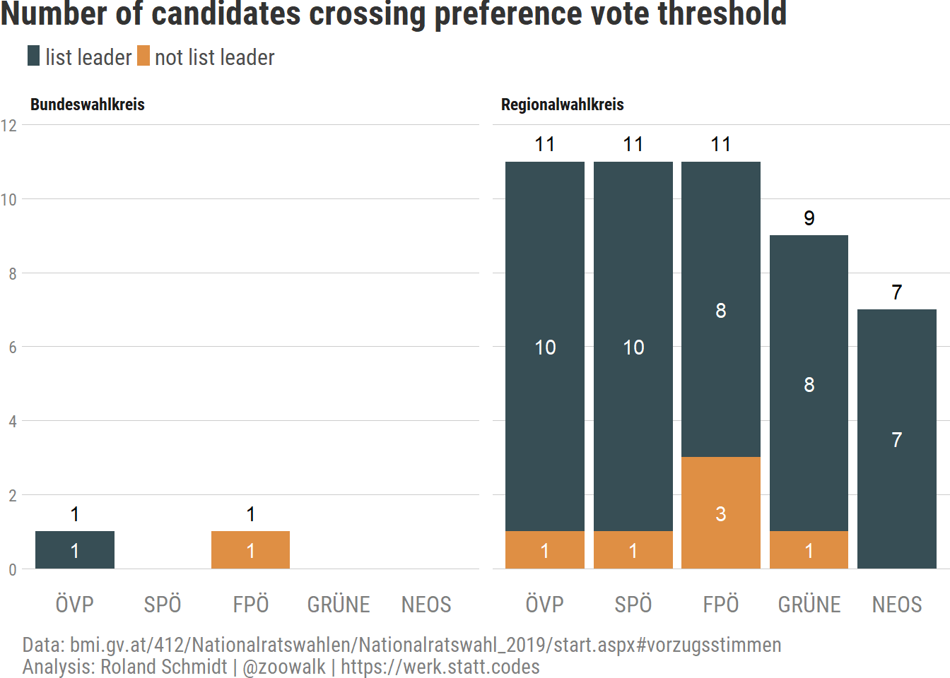
The graph below provides the number of candidates per party who were able to cross the required preference vote threshold. On the regional list level, ÖVP, SPÖ, and FPÖ had the same number of candidates, followed by the Greens and Neos. What the graph also reveals is that in the predominant part of cases, the successful candidates were in fact parties’ federal/regional list leaders. In total, only seven candidates which were not list leaders succeeded in securing the necessary preference votes. Probably noteworthy, 4 of these 7 cases originate from the FPÖ. Does this mean anything? I am tempted to suspect that parties with clear hiearchial structures are less likely to see lower rank candidates overtake their party’s list leaders. In cases, though, in which e.g. the leadership question is not entirely settled, or leaders are confronted with very strong ‘colleagues’ (Feind, Todfeind… Parteifreund), successful preference vote campaigns are more likely to occur. At least that’s an interpretation which came to my mind when seeing the numbers pertaining to the FPÖ (did I hear ‘selecting on the dependent variable’?). On the other hand, this proposition is immediately relativized when checking who these candidates were. With Kunasek (former Minister of Defense, leader of Styria’s FPÖ) and Haimbuchner (leader of Upper Austria’s FPÖ), we have two FPÖ representatives from the party’s upper echelons, who put their names on the ballot list, but - as far as I am aware - see their future as for now (again) in their home states rather than in the national parlament. I am only speculating here, but I found it at least noteworthy that the FPÖ somewhat deviates.
2.5.3 Difference Leader and Runners-up
Another angle to look at preference votes could be to examine the difference between the two candidates leading in terms of the number of preference votes. This gives us some idea on how dominant a candidate has been, i.e. whether the intra-party contestation at the top was particularly high. The graph above seeks to display the difference in candidates’ preference vote share per party and electoral district. Preference vote share is a candidate’s share of her party’s total preference votes in the respective list/constituency. Here, the higher the difference between those, the lower the contestation for the top spot. Hover over the dots to see the two top candidate and their respective share of preference votes. Not the small gap between SPÖ’s leader Rendi-Wagner and Mete.
2.5.4 Concentration of preference votes
Last but not least, to round off the picture, let’s see how different parties are when it comes to the concentration of preference votes. Are a party’s preference votes going almost exclusively to one or only a few candidates (high concentration)? Or, are preference votes relatively evenly shared among different candidates (low concentration)? A measure of concentration (Gini coefficient) can provide us with another angle on intra-party dynamics. Below the results:
3 Steps in R
Below some of the most important steps in R to obtain the results above. The full code is published on my github account here
3.1 Obtaining the preference vote results
The first potential hurdle is to virtually ‘liberate’ the results pertaining to the preference vote. Just have a look a the format of the data here and here. Particularly the results for the state and regional electoral district lists are not what a follower of ‘tidy data’ would hope for. So let’s start wrangling:
Code
# get state and regional list--------------------------------------

df_state_region <- readxl::read_xlsx(path = here::here("posts", "2019-11-20-vorzugsstimmen", "NRW19_Vorzugsstimmen_Landes_Regionalparteiliste_16102019.xlsx"))

names(df_state_region) <- names(df_state_region) %>%
  stringr::str_remove(., "\r") %>%
  stringr::str_remove(., "\n") %>%
  stringr::str_remove(., "-")

df_state_region <- df_state_region %>%
  janitor::clean_names()

df_state_region_long <- df_state_region %>%
  mutate(party = map_chr(reihung_1, ~ str_extract(., regex("^List.*")))) %>%
  mutate(state_list = map_chr(reihung_1, ~ str_extract(., regex("^Landespartei.*")))) %>%
  mutate(regional_list = map_chr(familien_vorname_2, ~ str_extract(., regex("^Regionalpartei.*")))) %>% # mess in bmi file; heading in different columns
  mutate(regional_list_2 = map_chr(reihung_1, ~ str_extract(., regex("^Regionalpartei.*")))) %>%
  mutate(district = coalesce(state_list, regional_list, regional_list_2)) %>%
  janitor::remove_empty("rows") %>%
  fill(., district, .direction = c("down")) %>%
  fill(., party, .direction = c("down")) %>%
  select(-c("x6", "state_list", "regional_list", "regional_list_2")) %>%
  filter(str_detect(reihung_1, "^[0-9]")) %>%
  select(district, party, everything()) %>%
  rename_at(
    vars(reihung_7:vorz_stimm_11),
    function(x) str_replace_all(x, "[:digit:]+", "b")
  ) %>%
  rename_at(
    vars(reihung_1:vorz_stimm_5),
    function(x) str_replace_all(x, "[:digit:]+", "a")
  ) %>%
  mutate_at(vars(reihung_a:vorz_stimm_b), as.character) %>%
  pivot_longer(
    cols = reihung_a:vorz_stimm_b, names_to = c(".value", "result"),
    names_pattern = "(.*)_([a|b]$)"
  ) %>%
  mutate_at(vars(reihung, geb_jahr, vorz_stimm), as.numeric) %>%
  group_by(district, party) %>%
  arrange(reihung, .by_group = T) %>%
  mutate(district_type = case_when(
    str_detect(district, regex("Landes.*")) ~ "Landeswahlkreis",
    str_detect(district, regex("^Regional.*")) ~ "Regionalwahlkreis",
    TRUE ~ NA_character_
  )) %>%
  select(district_type, district, party, everything(), -result) %>%
  rename(
    name = familien_vorname,
    pref_votes_abs = vorz_stimm,
    # district_type = district_type,
    # district = district,
    rank_list = reihung,
    birth_year = geb_jahr,
  ) %>%
  ungroup()


# get federal list --------------------------------------

df_federal <- readxl::read_xlsx(
  path=here::here("posts", "2019-11-20-vorzugsstimmen", "NRW19_Vorzugsstimmen_bundesweit_16102019.xlsx"),
  col_name = F,
  trim_ws = T
)

names(df_federal) <- c(
  "Nr", "Familienname, Vorname", "Geb.-Jahr", "Beruf",
  "Gesamt", "B", "K", "NÖ", "OÖ", "S", "Stmk", "Tirol",
  "Vlbg", "Wien"
)


df_federal_clean <- df_federal %>%
  janitor::remove_empty(., which = c("rows")) %>%
  filter(!Nr == "Nr.") %>%
  mutate(party = str_extract(Nr, regex("[:alpha:].*"))) %>%
  fill(., party, .direction = c("down")) %>%
  filter(!str_detect(Nr, regex("[:alpha:]"))) %>%
  mutate(district_type = "Bundeswahlkreis") %>%
  pivot_longer(cols = Gesamt:Wien, names_to = "district", values_to = "pref_votes_abs")


# rename to be consistent with regional/state level
df_federal_clean <- df_federal_clean %>%
  select(district_type, district, party,
    rank_list = "Nr", name = "Familienname, Vorname", birth_year = "Geb.-Jahr",
    beruf = "Beruf", everything()
  ) %>%
  mutate_at(vars("rank_list", "birth_year", "pref_votes_abs"), ~ stringr::str_trim(., side = c("both"))) %>%
  mutate_at(vars("rank_list", "birth_year", "pref_votes_abs"), as.numeric)


# bind both bund, laender and regio -------------------------------------------------------------------

df_merge <- bind_rows(
  df_state_region_long,
  df_federal_clean
) %>%
  ungroup() %>%
  filter(!is.na(name))

# write.csv2(df_merge,
#            file = paste0(wdr, "/data/AUT_NRW19_preference_votes.csv"),
#            row.names = F,
#            fileEncoding = "latin1"
# )


fn_remove_titles <- function(x) {
  titles <- c(
    "Mag", "MMag", "Prof", "Dr", "O\\.Univ\\.Prof", "Dipl-Ing", "Dipl.-Ing.", "Dipl.-Rev.", "Ing",
    "Dipl", "jun", "sen", "Ba", "\\(FH\\)", "MSc",
    "med", "univ", "Bsc", "phil", "iur", "DDr", "BEd", "DI", "Mba", "Mas", "MA", "MIM",
    "vet", "M.A.", "PMM", "MTD", "Päd", "Bakk"
  ) %>%
    map(., paste0, c("\\.", "\\s", "\\,")) %>%
    unlist()


  name_wo_titles <- stringr::str_remove_all(x, regex("[[:alpha:]\\-]+\\.")) %>%
    str_remove_all(., regex("\\([:alpha:]+\\)")) %>%
    str_remove_all(., regex(paste0(titles, collapse = "|"), ignore_case = T)) %>%
    str_squish()
}


fn_short_name <- function(x) {
  family_name <- stringr::str_extract(x, "^[[:alpha:]\\-|\\s]+(?=,)") %>%
    str_to_title() %>%
    str_squish() %>%
    str_trim()

  first_name <- str_extract(x, regex("(?<=\\,)[[:alpha:]\\-\\s]*$")) %>%
    str_trim() %>%
    str_squish() %>%
    str_to_title()

  initals <- str_split(first_name, "\\s") %>%
    map(., str_sub, start = 1L, end = 1L) %>%
    map_chr(., str_c, collapse = ".") %>%
    paste0(., ".")

  name_short <- paste(family_name, initals, sep = ", ")
}

df <- df_merge %>%
  mutate(district = str_remove(district, "Landesparteiliste") %>%
    str_remove(., "Regionalparteiliste") %>%
    str_trim(., side = c("both"))) %>%
  mutate(district = case_when(
    district == "B" ~ "Burgenland",
    district == "S" ~ "Salzburg",
    district == "K" ~ "Kärnten",
    district == "NÖ" ~ "Niederösterreich",
    district == "OÖ" ~ "Oberösterreich",
    district == "Stmk" ~ "Steiermark",
    district == "Vlbg" ~ "Vorarlberg",
    TRUE ~ district
  )) %>%
  mutate(district = as_factor(district)) %>%
  mutate(party2 = str_extract(party, regex("\\([:alpha:]*\\)")) %>% # take parties' short abbrevs.
    str_remove_all(., "\\(|\\)")) %>%
  mutate(name_orig = name) %>%
  mutate(name = map_chr(name_orig, fn_remove_titles)) %>%
  mutate(name_short = map_chr(name, fn_short_name)) %>%
  mutate(state = case_when(
    str_detect(district, "^[0-9].*") ~ str_sub(district, start = 1L, end = 1L),
    TRUE ~ as.character(district)
  )) %>%
  mutate(state = case_when(
    state == 1 ~ "Burgenland",
    state == 2 ~ "Kärnten",
    state == 3 ~ "Niederösterreich",
    state == 4 ~ "Oberösterreich",
    state == 5 ~ "Salzburg",
    state == 6 ~ "Steiermark",
    state == 7 ~ "Tirol",
    state == 8 ~ "Vorarlberg",
    state == 9 ~ "Wien",
    # TRUE ~ NA_character_
    TRUE ~ state,
  )) %>%
  mutate(district_type = fct_relevel(district_type, "Bundeswahlkreis", "Landeswahlkreis", "Regionalwahlkreis")) %>%
  mutate(name = case_when(
    str_detect(name, "Pistracher") ~ "Pistracher, Gerald",
    TRUE ~ as.character(name)))
Et voila (here only the first entries). If needed, you can downlaod the cleaned file here github repo.
If needed, you can download the cleaned file here from the github repo.
3.2 Abbreviating names, removing titles
An issue which has as been a frequent source of annoyance is the verbose use of academic and other (obviously even more important) titles in names. It only unnecessarily takes space from graphs and has something, in my personal view, deeply inegalitarian to it (the very purpose of using titles is probably to signal inegalitrianism). So, let’s remove all titles and only use the first letter of the first name. Regex and stringr are your friends here. Since this is a task which comes up time and again, it actually screams for a r package…
Code
fn_remove_titles <- function(x) {
  titles <- c(
    "Mag", "MMag", "Prof", "Dr", "O\\.Univ\\.Prof", "Dipl-Ing", "Dipl.-Ing.", "Dipl.-Rev.", "Ing",
    "Dipl", "jun", "sen", "Ba", "\\(FH\\)", "MSc",
    "med", "univ", "Bsc", "phil", "iur", "DDr", "BEd", "DI", "Mba", "Mas", "MA", "MIM",
    "vet", "M.A.", "PMM", "MTD", "Päd", "Bakk"
  ) %>%
    map(., paste0, c("\\.", "\\s", "\\,")) %>%
    unlist()


  name_wo_titles <- stringr::str_remove_all(x, regex("[[:alpha:]\\-]+\\.")) %>%
    str_remove_all(., regex("\\([:alpha:]+\\)")) %>%
    str_remove_all(., regex(paste0(titles, collapse = "|"), ignore_case = T)) %>%
    str_squish()
}


fn_short_name <- function(x) {
  family_name <- stringr::str_extract(x, "^[[:alpha:]\\-|\\s]+(?=,)") %>%
    str_to_title() %>%
    str_squish() %>%
    str_trim()

  first_name <- str_extract(x, regex("(?<=\\,)[[:alpha:]\\-\\s]*$")) %>%
    str_trim() %>%
    str_squish() %>%
    str_to_title()

  initals <- str_split(first_name, "\\s") %>%
    map(., str_sub, start = 1L, end = 1L) %>%
    map_chr(., str_c, collapse = ".") %>%
    paste0(., ".")

  name_short <- paste(family_name, initals, sep = ", ")
}


df <- df_merge %>%
  mutate(district = str_remove(district, "Landesparteiliste") %>%
    str_remove(., "Regionalparteiliste") %>%
    str_trim(., side = c("both"))) %>%
  mutate(district = case_when(
    district == "B" ~ "Burgenland",
    district == "S" ~ "Salzburg",
    district == "K" ~ "Kärnten",
    district == "NÖ" ~ "Niederösterreich",
    district == "OÖ" ~ "Oberösterreich",
    district == "Stmk" ~ "Steiermark",
    district == "Vlbg" ~ "Vorarlberg",
    TRUE ~ district
  )) %>%
  mutate(district = as_factor(district)) %>%
  mutate(party2 = str_extract(party, regex("\\([:alpha:]*\\)")) %>% # take parties' short abbrevs.
    str_remove_all(., "\\(|\\)")) %>%
  mutate(name_orig = name) %>%
  mutate(name = map_chr(name_orig, fn_remove_titles)) %>%
  mutate(name_short = map_chr(name, fn_short_name)) %>%
  mutate(state = case_when(
    str_detect(district, "^[0-9].*") ~ str_sub(district, start = 1L, end = 1L),
    TRUE ~ as.character(district)
  )) %>%
  mutate(state = case_when(
    state == 1 ~ "Burgenland",
    state == 2 ~ "Kärnten",
    state == 3 ~ "Niederösterreich",
    state == 4 ~ "Oberösterreich",
    state == 5 ~ "Salzburg",
    state == 6 ~ "Steiermark",
    state == 7 ~ "Tirol",
    state == 8 ~ "Vorarlberg",
    state == 9 ~ "Wien",
    TRUE ~ NA_character_
  )) %>%
  mutate(district_type = fct_relevel(district_type, "Bundeswahlkreis", "Landeswahlkreis", "Regionalwahlkreis"))
With the above we are basically ready to roll and start analyzing the data in earnest. The code below gives you the first plot (preference votes by district lists).
3.3 Plot - Total number of preference votes per electoral district
Code
df_list <- df %>%
  filter(!(district_type == "Bundeswahlkreis" & district != "Gesamt")) %>%
  group_by(district_type) %>%
  summarise(district_type_votes = sum(pref_votes_abs, na.rm = T)) %>%
  #  arrange(desc(district_type_votes)) %>%
  mutate(district_type = forcats::fct_relevel(district_type, "Regionalwahlkreis", "Landeswahlkreis", "Bundeswahlkreis")) %>%
  mutate(district_type_votes_cum = cumsum(district_type_votes)) %>%
  mutate(district_type_votes_perc = district_type_votes / sum(district_type_votes)) %>%
  mutate(district_type = forcats::fct_reorder(district_type, district_type_votes_cum, .desc = F))

pl_by_district <- df_list %>%
  ggplot() +
  geom_bar(aes(
    x = 1,
    y = district_type_votes,
    fill = district_type,
    group = district_type
  ),
  stat = "identity"
  ) +
  geom_text(aes(
    x = 1,
    y = district_type_votes,
    group = district_type,
    label = paste(scales::comma(district_type_votes),
      scales::percent(district_type_votes_perc),
      sep = "\n"
    )
  ),
  colour = "white",
  position = position_stack(vjust = .5, reverse = F)
  ) +
  scale_y_continuous(
    expand = expansion(mult = c(0, 0.05)),
    breaks = max(df_list$district_type_votes_cum),
    label = scales::comma(max(df_list$district_type_votes_cum))
  ) +
  scale_fill_paletteer_d("ggsci::default_jama",
    labels = c(
      "Regionalwahlkreis" = "Regional lists",
      "Landeswahlkreis" = "State lists",
      "Bundeswahlkreis" = "Federal list"
    )
  ) +
  labs(
    title = "Total number of preference votes per electoral district",
    caption = my_caption_2,
    y = "number of preference votes"
  ) +

  # hrbrthemes::theme_ipsum_tw() +
  # theme(
  #   plot.background = element_rect(fill=)
  #   legend.position = "top",
  #   legend.justification = "left",
  #   plot.title.position = "plot",
  #   legend.title = element_blank(),
  #   axis.text.y = element_blank(),
  #   axis.title.y = element_blank(),
  #   plot.title = element_text(size = 13),
  #   panel.grid = element_blank(),
  #   plot.caption = element_markdown(hjust = c(0, 1), color = "grey30"),
  #   plot.margin = margin(t = 0, l = 0, b = 0, r = 1, unit = "cm")
  # ) +
  coord_flip() +
  guides(fill = guide_legend(reverse = T))+
  theme_post()+
  theme(legend.position="top",
        legend.justification = "left",
        legend.direction  = "horizontal",
        plot.caption =element_text(hjust=0),
        # plot.background=element_rect(fill = "plot_bg_color", color="plot_bg_color"),
        legend.title = element_blank(),
        axis.text.y = element_blank(),
        panel.grid.major.y = element_blank()

        )
3.4 Group_split, map, and ggplot
Another part of the code which I’d like to highlight is the one producing the plot on candidates’ preference votes share. Here, rather than using a facet_grid, I split the dataframe by the electoral district lists, and mapped the plot function to each of the three parts, and subsequently combined them with patchwork. The advantage was that graph is more efficient in using the available space.
Code
share <- df %>%
  filter(!party2 == "Other") %>%
  filter(!(district_type == "Bundeswahlkreis" & district != "Gesamt")) %>%
  filter(!is.na(pref_votes_abs)) %>%
  group_by(district_type, state, district, party2) %>%
  arrange(desc(pref_votes_abs), .by_group = T) %>%
  mutate(index = row_number()) %>%
  mutate(sum_preference = sum(pref_votes_abs, na.rm = T)) %>%
  ungroup() %>%
  mutate(share_pref = pref_votes_abs / sum_preference) %>%
  # filter(share_pref>0.05) %>%  #change later
  left_join(., info_constituencies,
    by = c("district")
  )

df_thresholds <- tibble::tribble(
  ~threshold, ~district_type,
  .07, "Bundeswahlkreis",
  .10, "Landeswahlkreis",
  .14, "Regionalwahlkreis"
)

df_thresholds_2 <- crossing(df_thresholds, unique(share$party3)) %>%
  rename(party3 = `unique(share$party3)`)


df_share <- share %>%
  left_join(., df_thresholds_2,
    by = c("party3", "district_type")
  ) %>%
  mutate(share_pref = share_pref * 100) %>%
  left_join(., electoral_number %>%
    select(district_name, electoral_number),
  by = c("district" = "district_name")
  ) %>%
  mutate(electoral_number_indicator = case_when(
    pref_votes_abs > electoral_number ~ "yes",
    TRUE ~ as.character("no")
  )) %>%
  mutate(district_name=case_when(district_name=="Gesamt" ~ "Österreich",
                                 TRUE ~ as.character(district_name))) %>%
  left_join(., df_results %>% select(district_type, -district_name, district, party, votes_abs) %>%
              mutate(party=as_factor(party)),
              by=c("district_type"="district_type",
               #  "district_name"="district_name",
                 "district"="district",
                 "party3"="party")) %>%
  mutate(c_pvpv_ratio=round(pref_votes_abs/votes_abs, 4)) %>%  #c_pvpv candidates' preference vote vote ratio
  mutate(party3=as_factor(party3)) %>%
  ungroup() %>%
  mutate(sorting_index=group_indices(., district))


x <- df_share %>%
  select(district, district_name_short, sorting_index) %>%
  distinct()


plot_c_pvpv_ratio <- df_share %>%
  filter(party3 != "Other") %>%
  group_split(district_type) %>%
  map(~ ggplot(.) +
    labs(
      title = paste(unique(.$district_type)),
      subtitle = paste("Candidates securing preference votes more than
                    <span style='color:orange'>", unique(.$threshold) * 100, "</span> % of their party's overall vote in their respective constituency are re-ranked."),
      x = "Candidate's preference votes in % of party votes (C-PVPV)"
    ) +
    geom_point_interactive(aes(
      y = reorder(district_name_short, sorting_index),
      x = c_pvpv_ratio*100,
      # shape = as_factor(electoral_number_indicator),
      color = party3,
      data_id = name_short,
      tooltip = paste(name_short, round(c_pvpv_ratio*100, 2), sep = "; ")
    ),
    position = position_jitter(width = 0, height = 0.2, seed = 2),
    stat = "identity"
    ) +
    geom_vline(aes(xintercept = threshold * 100),
      color = "firebrick"
    ) +
    scale_y_discrete(expand = expansion(add = 0.2)) +
    scale_x_continuous(
      trans = "log10",
      limits = c(NA, 40),
      labels = scales::label_percent(accuracy = 1, scale = 1),
      minor_breaks = NULL,
      breaks = c(NA, 0, 1, 10, 40)
    ) +
    scale_color_manual(values = party_colors) +
    ggforce::facet_row(vars(party3),
      space = "free",
      scale = "free_x",
      shrink = T
    ) +
theme_post()+
    theme(
      axis.text.x = element_text(angle = 90, hjust = 1, vjust = .5, size = 9),
      axis.title.y = element_blank(),
      panel.spacing.x = unit(0.2, "cm"),
      panel.spacing.y = unit(0.2, "cm"),
      strip.text.x = element_text(
        angle = 0,
        vjust = 1,
        face = "bold"
      ),
      strip.text.y = element_text(
        angle = 180,
        vjust = 1,
        face = "bold"
      ),
      strip.placement = "outside",
      plot.title = element_text(size = 11, face = "bold.italic",
                                margin=margin(b=0, unit="cm")),
      plot.subtitle = element_markdown(size = 11, color = "grey30",
                                       face="italic"),
      plot.title.position = "plot",
      legend.position = "bottom",
      legend.title = element_blank(),
      legend.justification = "right",
      panel.grid.major.y = element_blank(),
      plot.margin = margin(0, unit = "cm")
    ) +
    guides(color = "none"))

plot_c_pvpv_ratio <- (patchwork::wrap_plots(plot_c_pvpv_ratio, ncol = 1) &
  theme(plot.margin = margin(unit = "cm", 0))) +
  plot_annotation(
    title = "Candidates' preference votes v. party votes ratio (C-PVPV)",
    subtitle = "Candidates above vertical line move up the electoral list.",
    caption = my_caption,
    theme = theme(
      plot.title = element_text(family = "Roboto Condensed", size = 12,face = "bold"),
      plot.subtitle = element_text(family = "Roboto Condensed", size = 12,face = "plain")))+
      plot_layout(heights = c(1, 9, 39))
3.5 Obtaining district magnitude
A convenient way to get data on the districts’ magnitude (number of mandates) is to scrap the pertainnig data from the website of the Ministry of Interior. The rvestpackage´ is our reliable tool here.
Code
library(rvest, quietly = T, verbose = F, warn=F)

MoI_url <- "https://www.bmi.gv.at/412/Nationalratswahlen/Wahlkreiseinteilung.aspx"

n_mandates_regional_districts <- MoI_url %>%
  read_html() %>%
  html_nodes("table") %>%
  html_table() %>%
  map_df(., bind_rows)
3.6 Geo_facet
Finally, as the last item, I’d like to highlight the wonderful geo_fact package. Rather than plotting data to a map by means of different color (shades), the geo_facet package allows facets of a plot to be arranged (more or less) in accordance with the map of e.g. a country. Here, I first created a grid which approximates the position the Austria’s states (Bundesländer), i.e. state electoral districts. This grid is subsequently passed on to the faceting function used in an otherwise ordinary ggplot command. The result you saw above here. Sweet, isn’t ;-)
Gladly, the author of the geo_facet package offers users the possibility to submit new grids to be integrated into the package. Once I have polished the grid (e.g. add iso codes), I’ll submit it and you can use it by simply calling the grid’s name in the geo_facet function (update: the grid was submitted and now part of the package).
Code
library(geofacet)

aut_grid <- data.frame(
  row = c(1, 1, 1, 2, 2, 2, 2, 2, 3),
  col = c(3, 4, 5, 1, 2, 3, 4, 5, 4),
  code = c("Oberösterreich", "Niederösterreich", "Wien", "Vorarlberg", "Tirol", "Salzburg", "Steiermark", "Burgenland", "Kärnten"),
  name = c("Oberösterreich", "Niederösterreich", "Wien", "Vorarlberg", "Tirol", "Salzburg", "Steiermark", "Burgenland", "Kärnten")
)

state_electoral_number <- df %>%
  filter(party3 != "Other") %>%
  filter(district_type == "Landeswahlkreis") %>%
  left_join(.,
    electoral_number %>% select(district_name, electoral_number),
    by = c("district" = "district_name")
  ) %>%
  select(district_type, district, name_short, party3, electoral_number, pref_votes_abs)

state_electoral_number_plot <- state_electoral_number %>%
  ggplot() +
  labs(
    title = "Candidates' preference votes and electoral number",
    caption = my_caption_2,
    y = "Preference votes"
  ) +
  geom_point_interactive(aes(
    x = party3,
    color = party3,
    y = pref_votes_abs,
    tooltip = paste(
      party3, "\n",
      name_short, pref_votes_abs
    )
  ),
  position = position_jitter(width = 0.2, height = NULL, seed = 2)
  ) +
  geom_hline(aes(yintercept = electoral_number),
    color = "firebrick"
  ) +
  geom_text(aes(
    x = Inf, y = electoral_number,
    label = scales::comma(electoral_number)
  ),
  color = "firebrick",
  nudge_y = -3000,
  family = "Roboto Condensed",
  hjust = 1,
  check_overlap = T
  ) +
  scale_color_manual(values = party_colors) +
  scale_x_discrete(expand = expansion(mult = 0)) +
  scale_y_continuous(
    labels = scales::label_comma(),
    expand = expansion(mult = 0),
    limits = c(0, 35000),
    minor_breaks = NULL
  ) +
  hrbrthemes::theme_ipsum_rc() +
  theme(
    axis.title.x = element_blank(),
    axis.text.x = element_text(size = 9),
    panel.grid.major.x = element_blank(),
    strip.text.y = element_text(angle = 0, vjust = 1),
    legend.position = "none",
    plot.title = element_text(size = 12, face="bold.italic", margin=margin(b=0, unit="cm")),
    plot.title.position = "plot",
    plot.caption = element_markdown(hjust = c(0, 1), color = "grey30"),
    plot.margin = margin(0, r = 0.2, unit = "cm"),
    strip.background.x = element_rect(fill = "lightgrey"),
    panel.border = element_rect(color = "lightgrey", fill = "transparent")
  ) +
  facet_geo(~district, grid = aut_grid) +
  guides(color = "none")
Footnotes
Reportedly, Hofer’s ‘defeat’ to Kickl might be due to an administrative issue though. There was another FPÖ candidate with the family name Hofer running on the federal constituency list. When voters put only the candidate’s family name on the ballot to indicate their preference, it was not clear which Hofer was actually meant. As a consequence, these preference votes were reportedly ruled as invalid.↩︎
I assume that the literature on preference votes has already coined a term for this indicator, but for the limited analysis here I leave it with this.↩︎
There seems to be an issue with the hoover over effect on mobile devices. If anyone knows how to iron this out, please let me know.↩︎
By dividing the number of valid votes in a state level constituency by the number of the constituency’s available mandates one gets the ‘electoral number’↩︎
Reuse
Citation
BibTeX citation:
@online{schmidt2019,
  author = {Schmidt, Roland},
  title = {Austrian {General} {Elections} 2019: {Preference} Votes},
  date = {2019-11-20},
  url = {https://werk.statt.codes/posts/2019-11-20-vorzugsstimmen/},
  langid = {en}
}
For attribution, please cite this work as:
Schmidt, Roland. 2019. “Austrian General Elections 2019:
Preference Votes.” November 20. https://werk.statt.codes/posts/2019-11-20-vorzugsstimmen/.